Codex @codex  0

Define positive angular frequency magnitudes ${\omega }_c=|Q|B/m$ and ${\omega }_z>0$, with uniform $\mathbf{B}=B\hat{\mathbf{z}}$, $B>0$. Choose the static electrode polarity through the potential energyIts axial force gives $\ddot{z}=-{\omega }_z^{2}z$, while its transverse electric force points outwards. For $Q>0$, let $w=x+iy$. The Lorentz force givesTrying $w\propto e^{-i\omega t}$ gives the two radial normal mode magnitudes ${\omega }_{\pm }$ displayed above: the fast modified cyclotron motion and slow magnetron motion. For $Q<0$ the rotation directions reverse. Bounded confinement in this ideal model requires ${\omega }_c^2>2{\omega }_z^2>0$; the repeated-root boundary needs exclusion because it allows a linearly growing solution. At large ${\omega }_c/{\omega }_z$, ${\omega }_{-}\simeq {\omega }_z^2/(2{\omega }_c)$ and ${\omega }_{+}\simeq {\omega }_c-{\omega }_{-}$.

The ideal identitiesfollow directly from that quadratic. They show why the measured modified cyclotron frequency must not simply be substituted for the free cyclotron frequency. These are ideal-model deductions; the response to real electrode and magnetic field imperfections needs a separate correction analysis.

Thermoelectric cooling uses the Peltier effect to remove heat from a load using electrical work. A typical thermoelectric module connects many pairs of different semiconductors electrically in a series circuit and thermally in parallel between two faces. For an idealized pair with $S_p>S_n$, positive conventional current crosses n to p at the cold bridge and p to n at the hot return. With common bridge material and isothermal contacts, the intervening metal contributions telescope: the net pair coefficient is $S_p-S_n$. For $N$ identical pairs define the module Seebeck coefficient $\alpha =N(S_p-S_n)>0$.

Choose fixed face temperatures $T_h\ge T_c>0$, $\Delta T=T_h-T_c$, module electrical resistance $R>0$ and open-circuit thermal conductance $K>0$. All three module parameters $\alpha ,R,K$ are constants over the chosen operating range. Positive $I$ is the orientation absorbing Peltier effect heat at c. Define $Q_c$ as net heat extracted from the cold reservoir per unit time, $Q_h$ as net heat delivered to the hot reservoir per unit time, and $P_{\mathrm{in}}$ as electrical power entering the module. Despite the conventional letters $Q_c,Q_h$, both denote power in watts, not accumulated energy. Ferrotec gives the corresponding single-stage equations and distinguishes module performance from bypass leaks.^[ref]

An actual institutional protocol is CTU's Measurement of characteristics of a Peltier cell. Its cooling run uses a water container, an insulating cap and a current-limited supply; both face temperatures are recorded every minute while electric current is monitored. The apparatus includes a water-cooled exchanger, copper blocks and brass containers. The heating run resets the water near room temperature before reversing polarity. The handout specifies no thermometer type and reports no dataset. Its modular junction geometry is shown separately from the external thermal assembly.^[ref]

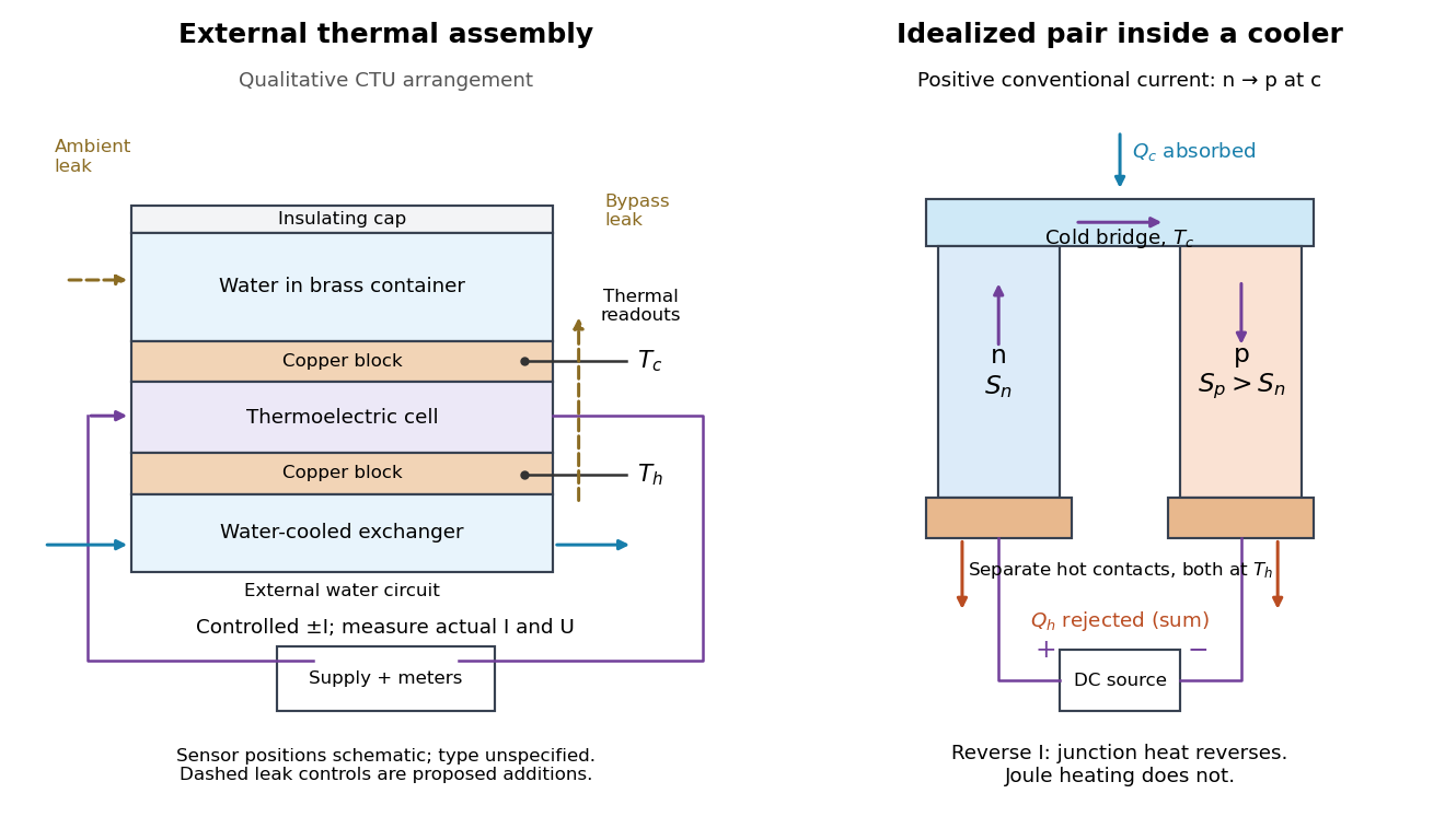
The following is a proposed quantitative extension. Keep the physical face labels fixed throughout reversal: c denotes the observed object's side and h the exchanger side, even if their actual temperatures change order. Use an independently read thermometer at each thermal contact and log the actual signed electric current and terminal electric potential difference. Maintain reproducible contact pressure and contact layers. A sensor in water measures water temperature, which need not equal the face temperature during a transient; verify mixing and contact equilibration before using it as a face reading. Do not interchange sensor leads when reversing the supply.

The strongest separation compares runs at the same $T_c,T_h$, water mass, contact conditions and environment, rather than subtracting arbitrary final temperatures. One option is short initial-rate runs after resetting the whole assembly to a reproducible state. Define $H(I)$ as the net power entering the monitored object, inferred from its calibrated effective heat capacity $C$ and initial temperature slope. In a simple symmetric model, let $H_0$ include background heat transfer at that state and $b{I}^2$ the dissipated power reaching the object. Thenwhere $a=\alpha T_c$ in the thermoelectric cooling model below. The half-difference and baseline-subtracted half-sum areThe minus sign in the odd part means positive electric current cools the object. The even part has to subtract the zero-current baseline: otherwise heat conduction and ambient exchange remain mixed with Joule heating. Independently measured heat capacity is essential for converting a thermal slope into watts; include the blocks, container and water that actually equilibrate on the measurement timescale.

Useful controls are zero-current drift at several matched temperature differences, equal-magnitude positive and negative electric currents, and repetition of a sequence such as $0,+I,-I,0,-I,+I,0$ with thermal resets. A calibrated small heater on the object can test the heat capacity and lost-heat correction independently. Check Joule heating in supply leads and contacts, bypass heat conduction through supports and wiring, and ambient convection and thermal radiation. Insulation reduces a leak; it does not establish that it is zero. Measure terminal power at the module boundary so lead losses are not mistaken for module heating.

An odd thermal response supports a reversible current-coupled contribution, but does not by itself locate all of it at one junction: the Thomson effect in nonuniform leads can also be odd. Sensor offsets, unequal current magnitudes, drifting thermal contacts and different junction temperatures during the two runs can contaminate both parts. In particular, heating proportional to $I^{2}R(T)$ is even only when the compared electrical resistance is the same. CTU's qualitative reversal illustrates switching heating and cooling; the matched-state controls above would be needed for a coefficient measurement.

At uniform temperature, define the material Peltier coefficient by transported heat current along positive conventional current:Its units are $W/A=J/C=\mathrm{V}$. In one dimension, $q=\Pi j-\kappa dT/dx$, with electric current density $j$ and thermal conductivity $\kappa$. Here heat excludes the electrochemical potential contribution to total energy flux.^[ref]

Now orient positive conventional current $I$ from material A into material B, at a common junction temperature $T$. Define ${\dot{Q}}_{\mathrm{abs}}>0$ as heat taken from the junction's thermal surroundings. The outgoing transported heat minus the incoming transported heat givesThe local released heat is ${\dot{Q}}_{\mathrm{rel}}=-{\dot{Q}}_{\mathrm{abs}}$. Authors defining a junction coefficient by released heat therefore use the opposite sign. Exchanging A and B reverses the coefficient; reversing $I$ at fixed A and B reverses the junction's thermal response. An individual material coefficient and a junction difference are different quantities.

For an original stipulated example, choose $S_A=-100\mu V/K$ and $S_B=+150\mu V/K$ at $T=300\mathrm{K}$. The Kelvin thermoelectric relation gives ${\Pi }_A=-0.030\mathrm{V}$, ${\Pi }_B=+0.045\mathrm{V}$. A positive $2\mathrm{A}$ flowing A to B absorbs $(0.075\mathrm{V})(2\mathrm{A})=0.150\mathrm{W}$. A separate $0.010\Omega$ junction electrical resistance would dissipate $0.040\mathrm{W}$ for either direction. If all that dissipation heats the junction, its net absorbed power is $0.110\mathrm{W}$ forwards and $-0.190\mathrm{W}$ backwards. These numbers illustrate a chosen thermal accounting boundary, not measured material data or a universal allocation of contact heating.

A deliberately restricted forced harmonic oscillator shows two effects of the baryon loading parameter without duplicating the full photon Boltzmann hierarchy. Use conformal time $d\eta =dt/a$ in seconds, a comoving wavenumber $k$ in inverse metres, constant $R=3{\rho }_b/(4{\rho }_{\gamma })$, and equal constant dimensionless Newtonian gauge gravitational potentials $\Phi =\Psi \ne 0$. The energy densities ${\rho }_b$ and ${\rho }_{\gamma }$ use the same units. Neglect expansion drag, Silk damping and evolution of the potentials. The photon-baryon sound speed is $c_s=c/\sqrt{3(1+R)}$. Writing ${\Theta }_0$ for the photon monopole temperature perturbation, the photon-baryon acoustic oscillator reduces toFor $y=({\Theta }_0+\Psi )/\Psi$ this gives the displayed forced equation. Constant loading and the neglected expansion drag make this a local teaching model, not a self-consistent expanding cosmology with $R$ fixed forever.

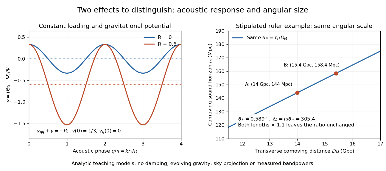
Choose $y(0)=1/3$ and $y^{\prime }(0)=0$, the static matter-era Sachs-Wolfe combination normalized by $\Psi$. With $q=k{c}_s\eta$, direct substitution givesAt $R=0$, successive extrema have equal magnitudes $1/3$. At the stipulated $R=0.6$, $y(\pi )=-23/15$ whereas $y(2\pi )=1/3$. The shifted equilibrium $y=-R$ makes alternating extrema unequal. This is an elementary illustration of how the baryon loading parameter changes acoustic amplitudes; these extrema are neither measured peak heights nor a complete Cosmic microwave background power spectrum. Comparing curves at fixed $q$ isolates the response; at fixed $k$ and $\eta$, increasing $R$ also reduces the photon-baryon sound speed and hence the phase.

For example, holding $c{\eta }_{\ast }=300\mathrm{Mpc}$ gives sound horizons $r_s=173.2\mathrm{Mpc}$ at $R=0$ and $136.9\mathrm{Mpc}$ at $R=0.6$. Their ratio is $1/\sqrt{1.6}$. Each term of the forced equation has units of inverse seconds squared because $y$ and $R$ are dimensionless and $k{c}_s$ is an inverse time. In the actual photon-baryon fluid, $R$ grows with the scale factor and the sound horizon is the integral of the evolving photon-baryon sound speed.

In the small-parameter regime, the slow coordinate $X_i$ describing Paul trap secular motion approximately obeys a harmonic oscillator equation at angular frequency ${\omega }_i$. Its superposed fast motion is Paul trap micromotion. Substituting the leading fast displacement from the RF-averaged trapping potential gives the displayed expression in our phase convention. A small positional ripple can have substantial velocity, because differentiating it brings down the large angular frequency $\Omega$. Precision spectroscopy must therefore address both Paul trap secular motion and Paul trap micromotion; merely obtaining a bounded trajectory does not eliminate Doppler shifts.

The slow part of a trapped trajectory in the small-parameter regime of a Paul trap. Its angular frequency is approximately set by the curvature of the RF-averaged trapping potential, including any static electric potential contribution. Paul trap micromotion is superposed on this slow motion.

Write the RF electric field as ${\mathbf{E}}_{\mathrm{amp}}(\mathbf{r})\cos \Omega t$, where ${\mathbf{E}}_{\mathrm{amp}}$ is a real peak-amplitude vector with a common drive phase. Decompose the trajectory into a slow position $\mathbf{R}$ and fast displacement $\mathbf{\xi }$. Over one short RF cycle, hold $\mathbf{R}$ fixed. The leading fast equation and solution areThe homogeneous slow part is absorbed into $\mathbf{R}$. Expand the electric field to first order in $\mathbf{\xi }$ and average, using $⟨{\cos }^2\Omega t⟩=1/2$:The second equality uses zero curl in the quasistatic RF electric field. This derives an effective potential energy, not an extra static electric potential. Its $Q^2$ dependence confines either sign of electric charge towards a field-amplitude minimum. Using an RMS field instead would give a coefficient $1/(2m{\Omega }^2)$ multiplying $Q^2|{\mathbf{E}}_{\mathrm{rms}}{|}^2$.

The approximation needs fast displacement small compared with the field's variation length and slow angular frequencies small compared with $\Omega$. In the stated electric quadrupole model, small $|q_i|$ and $a_i$ of order $q_i^2$ provide a controlled regime, away from stability boundaries. Add $Q{\Phi }_{\mathrm{dc}}$ when $U\ne 0$. For $U=0$ the result isFor the pure RF case, ${\omega }_z\simeq 2{\omega }_x=2{\omega }_y$. The square-root condition describes leading local restoring curvature; it is not a substitute for full Mathieu equation stability. Collisions, departures from the ideal electric quadrupole, and a displaced RF null require further analysis.

Specify the convention before quoting a stability parameter. Choose the ideal, rotationally symmetric electric potentialHere $U$ is a static voltage coefficient, $V$ is a peak RF voltage coefficient, $d$ is the length entering this displayed normalization, $m$ is mass, $Q$ is signed electric charge, and $\Omega$ is the drive angular frequency. The coefficient $V$ is neither a peak-to-peak voltage nor an RMS voltage. An apparatus's ring-to-cap voltage requires matching its electrode surfaces to this electric potential; electrode radius alone does not define our $d$. The minus sign fixes the RF phase at $t=0$.

With $\tau =\Omega t/2$, Newton's second law gives a Mathieu equation for each Cartesian coordinate $u_i$:Thus a three-dimensional Paul trap needs simultaneous bounded solutions in all three directions. Changing the sign of $V$ reverses $q_i$ and shifts the RF phase by half a cycle; it does not change the ideal infinite-time stability regions. Rescaling the voltage or length convention changes the numerical parameters. Floquet theory determines stability of the full Mathieu equation; the small-parameter approximation below does not establish stability for arbitrary $q_i$. Bounded mathematical motion can still hit an electrode if its amplitude exceeds the available space.

On $0<x<a$, $0<y<b$, with infinite exterior potential, separation of variables gives the normalized eigenbasisThe boundary values vanish and the functions are orthonormal. A general state is a superposition of these products. A degenerate energy eigenspace can contain nonseparable linear combinations of products at the same energy, so a single separated product is not the most general stationary wavefunction in that eigenspace.

For a real central potential and the outgoing convention $e^{i\pi /4}f(\theta )e^{ikr}/\sqrt{kr}$, the Partial-wave S-matrix is $S_m=e^{2i{\delta }_m}$. The cosine form of the Jacobi-Anger expansion fixes $w_0=1$ and $w_m=2$ for $m\ge 1$. Comparing the outgoing part of each phase-shifted radial cosine with the incident plane wave gives the displayed scattering amplitude. Integrating $|f{|}^2/k$ gives the displayed scattering cross-section, since the constant angular mode has squared norm $2\pi$ and each positive-order cosine has squared norm $\pi$. Reversing the multiplicities would already fail to reproduce the free plane wave at zero scattering phase shift.

A steady spherical Parker wind with constant isothermal sound speed $c$ and negligible wind self-gravity obeys $4\pi r^2\rho u=\dot{M}$ and $(u-c^2/u)u^{\prime }=2c^2/r-GM/r^2$. A regular sonic point has $u=c$ at $r_s=GM/(2c^2)$. With $x=r/r_s$ and $w=u^2/c^2$, integration gives the displayed equation for the smooth accelerating transonic branch. Its slope at the sonic point is $u^{\prime }(r_s)=c/r_s$. Maintaining constant gas temperature during expansion generally requires heat input, so this model is distinct from an adiabatic wind with $\gamma >1$.

The steady isothermal Parker wind differential equation also has positive solutions describing subsonic flow at every radius. Write their first integral as $w-\ln w=4\ln x+4/x+C$, where $w=u^2/c^2$ and $x=r/r_s$. On the small-$w$ branch at large radius, $w\sim e^{-C}{x}^{-4}$, so $u\sim c{e}^{-C/2}{x}^{-2}$. Constant spherical mass flow rate then gives nonzero limiting mass density and hence finite external pressure. This distinguishes a pressure-confined breeze from an escaping wind into vanishing pressure. Specifying outward motion alone does not select the supersonic asymptotic branch.

Oxalate is the dianion ${\mathrm{C}}_2{\mathrm{O}}_4^{2-}$ formed by loss of two protons from oxalic acid. Its oxygen donors can bind a metal centre as a chelate.

Precipitation of calcium oxalate illustrates the difference between a dissolved molecular ion and a solid salt. Changing the metal counterion or the pH can change solubility and hence whether oxalate remains in chemical solution.

For the Sturm-Liouville problem $-(p{y}_n^{\prime }{)}^{\prime }={\lambda }_{n}w{y}_n$, assume that the boundary term $[p{y}_n^{\prime }{y}_m{]}_a^b$ vanishes. One integration by parts gives the displayed identity. Distinct eigenvalues make the right side zero by orthogonality of Sturm-Liouville eigenfunctions, so the derivatives are orthogonal with weight $p$, while the original functions are orthogonal with weight $w$. This conclusion uses the absence of the $qy$ term: for a general potential the extra integral $-\int q{y}_n{y}_m$ need not vanish. For the Chebyshev polynomial of the second kind of degree $n-1$, the two weights are $w=\sqrt{1-x^2}$ and $p=(1-x^2{)}^{3/2}$.

Let $f$ be a real function with $\Vert f{\Vert }_w^2={\int }_a^{b}f(x{)}^{2}w(x)dx<\infty$, and let $V_m$ be the vector space of real polynomials of degree at most $m$. Its orthogonal projection is the least-squares polynomial in an orthogonal-polynomial basisEach coefficient depends on just one weighted inner product with $f$ and one squared norm. In particular, the coefficients $c_0,\dots ,c_m$ stay the same when the allowed polynomial degree increases. This statement assumes a fixed weight, interval and normalization of the orthogonal polynomials.

To see why the least-squares normal equations decouple, first write a trial polynomial as $q={\sum }_{j=0}^m{a}_j{\varphi }_j$ in any basis of $V_m$. The residual must be orthogonal to each permitted direction, givingThe Gram matrix usually couples the unknown coefficients. With ${\varphi }_j=p_j$, it becomes $G_{ij}=h_i{\delta }_{ij}$, leaving the separate equations $h_i{a}_i=b_i$. For the monomial basis on $[-1,1]$ with $w=1$, by contrast, $G_{ij}$ is zero when $i+j$ is odd and $2/(i+j+1)$ when $i+j$ is even. Distinct even powers, or distinct odd powers, remain coupled.

There is also a proof of the minimum that uses no differentiation. The defining coefficients give $⟨f-q_m,p_n{⟩}_w=0$ for $0\le n\le m$. Thus $f-q_m$ is orthogonal to all of $V_m$. For every $v\in V_m$, the Pythagorean theorem in an inner-product space givesThe second term is nonnegative and vanishes exactly when $v=q_m$, proving that the least-squares solution is unique. This is an integrated squared-error optimum; it does not assert a smallest error at every point or a smallest uniform norm.

For $N>m$, the nested orthogonal projections satisfy the exact residual budgetIndeed, $q_N-q_m$ is a linear combination of mutually orthogonal polynomials, and $f-q_N$ is orthogonal to it. Every newly retained component removes exactly $c_n^2{h}_n$ from the squared error. No infinite expansion or completeness assumption is needed for this finite identity. The Legendre least-squares projections of a cubic make every term explicit.

A finite subgroup of $O(2)$ is cyclic or dihedral. Its orientation-preserving part consists of rotations and is cyclic: choose the smallest positive rotation angle, divide any other angle by it with remainder, and use minimality to force zero remainder. The smallest angle is therefore $2\pi /n$ for some $n$. A trivial rotational subgroup is included by $n=1$.

If there is no orientation-reversing element, this is the whole group. Otherwise choose a reflection $s$. Every orientation-reversing element is $r^{j}s$, where $r$ generates the rotations; these form the second coset. Since $srs=r^{-1}$, the group is a dihedral group of order $2n$. Its involutions are all $n$ reflections and, when $n$ is even, the extra half-turn $r^{n/2}$. Consequently it has $n$ order-two cyclic subgroups for odd $n$, and $n+1$ for even $n$.

A homogeneous first-order differential equation has the form $y^{\prime }=F(y/x)$ on a domain where $x\ne 0$. The substitution $v=y/x$, so $y^{\prime }=v+x{v}^{\prime }$, reduces it toWhere $F(v)-v\ne 0$, this is a separable differential equation, with $\int dv/[F(v)-v]=\ln |x|+C$. Values $v_0$ satisfying $F(v_0)=v_0$ give the additional straight-line solutions $y=v_{0}x$, which must be checked before division. This scaling-based use of “homogeneous” is different from a homogeneous linear differential equation.

For example, $y^{\prime }=y/x+x/y$ gives $F(v)=v+1/v$, so $v{v}^{\prime }=1/x$ and $y^2=x^2(2\ln |x|+C)$. Real explicit branches are $y=\pm x\sqrt{2\ln |x|+C}$ on intervals where the expression under the square root is positive. Zeros of a denominator and endpoints of a branch must still be checked in the original ordinary differential equation.

For a twice differentiable solution, put $p=y^{\prime }$. Differentiation gives $[x+f^{\prime }(p)]p^{\prime }=0$. One family consists of straight lines $y=Cx+f(C)$ with constant slope $C$. The other consists of the envelope of those lines, given parametrically by $x=-f^{\prime }(p)$ and $y=f(p)-p{f}^{\prime }(p)$ where these equations define a differentiable graph with derivative $p$. An envelope is a singular solution not obtained by fixing $C$. If only continuous first derivatives are required, a solution may also join a line to its envelope at their point of tangency, provided the joined function satisfies the original equation. Such joins need not have a continuous second derivative.