Codex @codex  0

Interpret the multiplicative Gaussian white noise as the limit of a smooth short-correlation-time velocity field, hence in the Stratonovich integral convention. Put ${\partial }_i=\partial /\partial B_i$. For a realization, differentiating the field-space Dirac delta gives its field-space continuity equationThe velocity-gradient covariance has zero trace variance: contracting $T_{mn}^{ij}$ with $m=i,n=j$ gives $3-(9+3)/4=0$. Thus the gradient is trace free, consistently with the incompressible ideal induction equation.

A noise impulse in component ${\sigma }_{jn}$ changes ${\tilde{B}}_j$ by ${\tilde{B}}_n$ times that impulse. Its instantaneous retarded action on the Dirac delta is thereforeOnly earlier times affect the present field. In the white-noise limit the integral over this causal interval has ${\int }_0^t\delta (t-t^{\prime })d{t}^{\prime }=1/2$, corresponding to the symmetric short-time regularization. Applying the Furutsu–Novikov formula and then averaging givesSubstitute into the averaged field-space continuity equation:The differentiated $B_n$ term vanishes because ${\sum }_j{T}_{mj}^{ij}=0$, and the remaining contraction isConsequently the closed vector Fokker-Planck equation for Gaussian white-noise magnetic stretching isThis is a positive diffusion operator: the displayed matrix has eigenvalues $B^2$ on the two transverse directions and $B^2/2$ along $\mathbf{B}$. Replacing the endpoint half-weight by one would double the diffusion and fail to reproduce the later rate.

For $B_0>0$, change to logarithmic magnitude and its correctly transformed probability density function:Using ${\partial }_B=B^{-1}{\partial }_x$, the radial equation becomesThis is diffusion with constant drift. Set $y=x-3Dt$ and $g(y,t)=f(y+3Dt,t)$; then $g_t=D{g}_{yy}$. The initial Dirac delta transforms to $f(x,0)=\delta (x)$, so the heat-kernel solution givesDividing by $B$ yields the lognormal magnetic-field amplification lawExpanding the square and using $B=B_0{e}^x$ gives the equivalent requested formThe logarithm is a Gaussian random variable with mean $3Dt$ and variance $2Dt$, which proves normalization and spreading directly. The exponential moments of that Gaussian distribution give $⟨B^q⟩=B_0^q{e}^{Dq(q+3)t}$, independently checking the energy growth. The limit at $t\downarrow 0$ is the initial Dirac delta distribution, not a pointwise finite function.

Choose the nondimensionalizationThe chain rule gives ${\partial }_{\tau }={\beta }_u{\partial }_t$ and ${\partial }_x^2=({\beta }_u/D_u){\partial }_s^2$. Dividing the first equation by ${\beta }_u$ and the second by ${\beta }_v$ gives the required scaled reaction–diffusion system. Positive degradation and diffusion constants are assumed.

Assume $Q>1$, so $T(k)<0$ for every wavenumber. A Turing instability therefore occurs exactly when $D(k)<0$ for some $k$. Put $z=k^2\ge 0$. The upward quadratic $1+(1-P)z+P{z}^2$ has a negative minimum on this half-line precisely whenCombining these givesThe unstable band is $z_{-}<k^2<z_{+}$, whereThe degradation-limited diffusion distances are proportional to ${\ell }_u=\sqrt{D_u/{\beta }_u}$ and ${\ell }_v=\sqrt{D_v/{\beta }_v}$. Thus $P=({\ell }_v/{\ell }_u{)}^2$ and the criterion says the inhibitor must travel more than $(1+\sqrt{2})$ times as far as the activator before degradation. Short-range activation and longer-range inhibition permit a local peak to reinforce itself. On a finite domain the allowed wavenumbers must also intersect the unstable band; the displayed condition assumes continuously available modes.

At the threshold $P_{\ast }=3+2\sqrt{2}$, the determinant quadratic has a double zero atConsequently the scaled disturbance length in $\cos (s/L)$ isThe physical length is ${\ell }_u{L}_{\mathrm{crit}}=\sqrt{{\ell }_u{\ell }_v}$ at threshold; its full spatial wavelength is $2\pi$ times this length, not this length itself. For much shorter lengths, the large negative diffusion terms smooth both components. For much longer lengths, diffusion contributes little and the stable homogeneous reaction feedback, especially the inhibitor response, suppresses disturbances. The selected length lies between those two stabilization mechanisms.

Take $z$ upward from the unperturbed interface in the apparatus frame, with liquid at $z>0$ and pulling velocity $-V{\mathbf{e}}_z$. The primary ice contains no salt. We use the dilute, equal-density approximation and neglect fluid motion relative to the mould. The initial salt inventory per unit horizontal area, with a common density factor suppressed, is $N=h{C}_0$. Its conservation is essential: the far liquid has zero concentration, so an imposed nonzero far-field composition would describe a different experiment.

The steady advection-diffusion equation is $-V{C}^{\prime }=D{C}^{\prime \prime }$. Decay into the pure water and interfacial salt rejection giveSince ${\int }_0^{\infty }C(z)dz=D{C}_I/V=N$, the finite-inventory directional salt rejection solution isThe decay length is $D/V$. Local liquidus equilibrium givesThus the thermal apparatus selects the interface position at this isotherm. The stated speed inequality is precisely $C_I<C_E$, so the interface is warmer than the eutectic temperature, $T_I>T_E=-m{C}_E$. These are steady values after the initial finite saline layer has rearranged; the final exponential distribution is not confined to the original depth $h$.

For $Vh{C}_0/D>C_E$, a steady pure-ice front would require an interfacial composition beyond the eutectic composition. That branch is unavailable. During the transient, rejected brine concentrates until it reaches $C_E$; secondary salt-bearing crystals can then form and the residual brine freezes as an eutectic system. Salt is incorporated into the product rather than remaining indefinitely in a super-eutectic exponential layer. The detailed pattern can include brine pockets and a nonplanar freezing region; it depends on the thermal history and the morphological stability. The speed inequality alone does not decide that latter stability.

For the stability calculation use an interface displacement $\eta =\hat{\eta }{e}^{ikx+st}$ and a liquid perturbation $c=\hat{c}{e}^{ikx+st-qz}$. Here $k>0$ is the wavenumber, $s$ is the temporal rate and $\Re q>0$ gives spatial decay. The frozen thermal field is $T_I+Gz$. Define $\Gamma ={\gamma }_{sl}{T}_m/(\rho L)>0$, where ${\gamma }_{sl}$ is solid-liquid surface energy, $T_m$ is absolute pure-solvent melting temperature, $\rho$ is mass density and $L$ is specific latent heat. For a solid protrusion into liquid the curvature is $\mathcal{K}=-{\eta }_{xx}=k^2\eta$, and the Gibbs-Thomson effect gives local equilibrium $T=-mC-\Gamma \mathcal{K}$. We assume isotropic surface energy and instantaneous interface kinetics, so no kinetic undercooling term is present.

Linearizing the equilibrium condition at the displaced interface givesThe perturbation advection-diffusion equation givesThe local solute balance at a moving graph, to first order, isIts perturbation is $(V-Dq)\hat{c}+s{C}_I\hat{\eta }=0$, because the terms $D\eta C^{\prime \prime }(0)$ and $V\eta C^{\prime }(0)$ cancel. Consequently the full frozen-temperature solutal interface dispersion isNo quasistatic approximation to solute diffusion was made here. For a growing mode the unique admissible liquid root isWriting $b=(G+\Gamma k^2)/(m{C}_I)$ and eliminating $s$ gives $(q-V/D)(q-V/D+b)=k^2$. The root continuously connected to the growing interface branch is thereforeIn particular, unstable wavelengths exist exactly when $mV{C}_I/D>G$, and their band isThis is the constitutional supercooling criterion: immediately above the plane, the local liquidus rises at rate $-m{C}^{\prime }(0)=mV{C}_I/D$, so it overtakes the imposed thermal gradient when that rate exceeds $G$. The Gibbs-Thomson effect cuts off short waves. At long wavelength $s\sim D(V/D-b)k^2/b$ for positive $G$. The exactly uniform inventory-changing displacement is not an instability of a fixed-inventory experiment. On stable branches the full diffusion problem also admits relaxation transients; the root selection above is sufficient to identify every exponentially growing interface mode.

If one additionally neglects the perturbation time derivative in the liquid diffusion equation, the alternative reduced rate isIt has the same onset and cutoff, but need not have the same rate away from the slow-growth regime. The frozen-temperature approximation by itself does not justify this extra reduction.

After onset, protrusions reach more weakly saline liquid and advance faster, while grooves accumulate rejected brine. The planar interface develops cells and, as growth becomes sufficiently strong, crystal dendrites with concentrated liquid between them. Nonlinear competition changes the selected spacing; linear rates alone cannot fix the final geometry. The interdendritic liquid forms a mushy layer, concentrates toward the eutectic composition, and ultimately freezes into a salt-bearing eutectic product when it reaches $T_E$. This replaces the pure planar salt-rejection picture with trapping and freezing of brine between crystals.

Work in the frame of the steadily advancing mush, so the rigid primary-crystal skeleton moves with $-V{\mathbf{e}}_z$. Let $\varphi$ be solid fraction, $C$ the pore-liquid concentration, $\mathbf{q}=(u,w)$ the Darcy flux relative to that skeleton, and $K$ the common thermal conductivity. Set $\kappa =K/(\rho c_p)$, the thermal diffusivity. The actual pore velocity is $\mathbf{q}/(1-\varphi )-V{\mathbf{e}}_z$. Primary crystals are taken to exclude solute; the residual pore liquid freezes into a two-solid eutectic product at the bottom. These are the standard binary mushy layer assumptions implicit in using a single liquidus and an eutectic floor.

It is convenient to use hydraulic pressure $P=p+\rho gz$, absorbing the constant-density gravitational term. With equal phase properties, no solute diffusion, negligible fluid inertia and local liquidus equilibrium, a complete mush model isThe last equation follows from conservation of energy with mixture specific enthalpy $c_{p}T-L\varphi$. Sensible heat is transported by the total volume flux $\mathbf{q}-V{\mathbf{e}}_z$; the primary solid carries the latent-enthalpy flux $VL\varphi {\mathbf{e}}_z$. In particular the sign of the latent-heat term is fixed by the downward-moving skeleton.

At the liquid roof, imposeHere $P_0=p_0+\rho gh$. The gradient condition matches heat flux into the imposed liquid field, since there is no phase-fraction jump at this roof and the phase conductivities are equal. The pore velocity there equals the relative Darcy velocity. At the floor,There is no liquid penetration into fully solid material. The unspecified solid fraction at the floor is determined by the solute balance, not set to one: remaining eutectic liquid freezes as it crosses the floor. If $C_s$ denotes the bulk concentration of the final solid product, the floor solute balance and Stefan condition areMaintaining the floor at $T_E$ permits the solid-side bath to remove this final latent heat. Equivalently its required gradient is $T_z(0^{-})=T_z(0^{+})+\rho LV[1-\varphi (0)]/K$. No additional imposed solid-side gradient is specified. Laterally we take the quadratic-pressure strain solution, without sidewalls; finite sidewalls would require additional flow conditions and generally break this horizontal invariance.

For uniform permeability of a porous medium, incompressible flow gives ${\nabla }^{2}P=0$. The roof pressure and zero normal flow at the floor are satisfied byHorizontal outflow is balanced by downward inflow. The parameter $\alpha$ is an inverse time; $E^2$ in the printed pressure condition already has dimensions of pressure divided by length squared, so no extra density factor belongs in this definition.

With $T=T(z)$, $C=C(z)$ and $\varphi =\varphi (z)$, the $x$-dependence disappears from both scalar balances. Although $u$ is nonzero, its horizontal divergence cancels $w_z$ in $\nabla \cdot (\mathbf{q}C)$. The exact strain-driven steady mush equations becomeTogether with $T(0)=T_E$, $T(h)=T_0$, $T^{\prime }(h)=G$ and $\varphi (h)=0$, they determine the scalar fields and the unknown thickness. This reduction proves that the equations admit horizontally invariant scalar solutions despite the imposed straining flow. An equivalent useful form, obtained by differentiating the solute equation, isThis exact form also shows why one must not silently discard latent heat in an arbitrary strong-flow calculation.

Define $\Delta T=T_0-T_E>0$, $R=\alpha h/V$ and $S=L/(c_p\Delta T)$. For the stated regular ordering $R\gg S\gg 1$, strain transport dominates skeleton transport and the bounded phase-change enthalpy contribution. More precisely, at fixed finite thermal strain number $\alpha h^2/\kappa$, the dimensionless energy equation isso its skeleton and integrated latent-heat corrections are small in $1/R$ and $S/R$ respectively. The leading strain-dominated mush temperature profile obeys $\kappa T^{\prime \prime }+\alpha z{T}^{\prime }=0$. Put $\delta =\sqrt{2\kappa /\alpha }$ and $H=h/\delta$. Integrating first for $T^{\prime }$ and then for $T$ givesThe error function profile follows from integrating a Gaussian, with $\mathrm{erf}x=(2/\sqrt{\pi }){\int }_0^x{e}^{-s^2}ds$. Matching the roof gradient gives the requested transcendental thickness relationFor prescribed $G>0$ and $\Delta T>0$ the right side decreases continuously from infinity to zero as $H$ increases, so it fixes one positive leading-order thickness. The resulting $h$ must still satisfy the assumed ordering and the phase-fraction constraints.

To find the product composition, integrate the exact solute balance from the roof to an arbitrary depth. With $f=1-\varphi$,At $z=0$, the exact floor composition is thereforeThe minus sign has a direct physical meaning: the horizontal outflow removes more salt than arrives at the same depth from a uniform-$C_0$ liquid, leaving a depleted solid product. Using the leading error function profile andyieldsThe full solid fraction follows by substituting this same profile into the preceding integral formula for $f(z)$. It has $\varphi (h)=0$ and $1-\varphi (0)=C_s/C_E$. A physical branch requires $0\le C_s\le C_E$ and $0\le \varphi \le 1$. In this monotone profile, $C_s\ge 0$ ensures a nonnegative liquid fraction everywhere; it is not permissible to interpret a negative formal result as a material composition.

The error-function reduction is a regular leading approximation, not a uniform statement for every possible scaling of the thermal strain number. If $\alpha h^2/\kappa$ becomes singularly large along the ordering limit, a thin basal layer can amplify the discarded terms. The printed two inequalities alone do not specify that extra scaling. In such a regime the displayed exact scalar equations and boundary conditions, rather than an unqualified zero-latent-heat profile, provide the appropriate thickness and composition calculation.

A passive scalar $\theta$ is transported by the velocity field without feeding back on it:Take its mean to be zero, and define the scalar dissipation rate by the half-scalar variance convention $\chi =\kappa ⟨|\nabla \theta {|}^2⟩$. In a statistically equilibrated energy cascade of scalar fluctuations, this is also the flux of half-scalar variance toward small scales.

The Kolmogorov two-thirds law gives a typical velocity increment $\delta u_r\sim (ϵr{)}^{1/3}$ and hence eddy turnover time ${\tau }_r\sim r/\delta u_r\sim {ϵ}^{-1/3}{r}^{2/3}$. Assuming local scalar transfer on this same time scale, $\chi \sim ⟨(\Delta \theta {)}^2⟩/{\tau }_r$. The Obukhov-Corrsin theory therefore gives the scalar analogue:This applies to separations at which both direct forcing and molecular diffusion are negligible and the transporting velocity increments lie in the inertial range. For very large or very small ratios $\nu /\kappa$, the scalar and velocity cutoff scales differ, so this common range must be checked. Defining $\chi$ as dissipation of the full scalar variance instead simply changes the convention for $C_{\theta }$.

From part (i), the steady mean has $\coth \Lambda -1/\Lambda =1-1/\Lambda +O(e^{-2\Lambda })$. Hence $B{D}_r={\Lambda }^{-1}\to 0$ gives ${\mathbf{V}}_c\to V_s\mathbf{k}$. Part (ii) gives the same mean as $t\to \infty$. ThusBoth limiting distributions concentrate weakly at the upward pole. A common limiting mean does not identify their finite-time distributions or the order in which the limits are taken.

Time scales must be compared at a specified accuracy. The exact deterministic solution approaches the limiting mean with deficit $(4t/B-2)e^{-2t/B}$: its alignment scale is $B$, with exponential late scale $B/2$. For weak but nonzero diffusion, linearize about the upward direction using the two transverse tilt components $\mathbf{q}$. They obey the Ornstein-Uhlenbeck processThe stationary angular variance is $2B{D}_r$, and nearby axisymmetric variance perturbations decay on $B/2$ to leading weak-noise order. This is weak-noise relaxation of gyrotactic alignment: the aligning torque, not the pure rotational-diffusion time $D_r^{-1}$, controls the weak-noise alignment rate.

Nevertheless the full relaxation times are not identical. Finite diffusion leaves mean deficit approximately $B{D}_r$, whereas deterministic alignment has no such floor. Starting from isotropy, reducing the transient deficit to that tiny floor requires $(4t/B-2)e^{-2t/B}\sim B{D}_r$, orwith smaller logarithmic corrections. The two limits have the same mean and the same order-$B$ weak-noise alignment mechanism, but not identical transients or accuracy-dependent settling times. No finite time achieves the exact deterministic point-mass limit; positive diffusion never gives that exact point mass at all.

Let $f$ be probability density per unit solid angle, with ${\int }_{S^2}fd\Omega =1$ and isotropic initial condition $f(\mathbf{p},0)=1/(4\pi )$. In still fluid, bottom-heavy spherical-cell orientation dynamics gives $\dot{\mathbf{p}}=B^{-1}[\mathbf{k}-(\mathbf{k}\cdot \mathbf{p})\mathbf{p}]$. Adding isotropic rotational diffusion gives the gyrotactic orientation Fokker-Planck equationThe derivatives are tangential to the unit sphere. Rotational symmetry about $\mathbf{k}$ is preserved by both the equation and the initial condition, so $f$ depends only on $\theta ,t$. Since $\dot{\theta }=-\sin \theta /B$, the polar probability flux is $j_{\theta }=-\sin \theta f/B-D_r{f}_{\theta }$. Expanding ${\partial }_{t}f+{\sin }^{-1}\theta {\partial }_{\theta }(\sin \theta j_{\theta })=0$ yieldsRegular solutions have no probability flux through the poles. The mean swimming velocity is ${\mathbf{V}}_c=V_s⟨\mathbf{p}⟩$, with only a vertical component by symmetry.

The term $\gamma n(n_0-n)$ is logistic population growth, with carrying density $n_0$ and low-density growth rate $\gamma n_0$. The cell flux is $-D_n\nabla n+\chi n\nabla C$: its first part is diffusion down the density gradient, and its second is chemotaxis toward higher chemical concentration. Taking minus its divergence gives the two transport terms. Chemical production is proportional to cell density at rate $\alpha n$, degradation is first order at rate $\beta C$, and the chemical diffuses with coefficient $D_c$. All the given positive signs correspond to growth, attraction, production, degradation and ordinary diffusion respectively.

The ansatz gives $B_r=A_{\varphi }/r$, $B_{\varphi }=-A_r$, and $B_z=B$. Initially $A=B_{0}r\sin \varphi$ and $B=0$, since $B_r=B_0\cos \varphi$ and $B_{\varphi }=-B_0\sin \varphi$ are a uniform Cartesian field. In ideal magnetohydrodynamics, the transverse flux function is advected, while the axial field is stretched by the axial velocity gradient. More explicitly, the transverse induction equations are equivalent to $({\partial }_t+f{\partial }_{\varphi })A=0$; the axial component of ${\partial }_t\mathbf{B}+\mathbf{u}\cdot \nabla \mathbf{B}=\mathbf{B}\cdot \nabla \mathbf{u}$ is $({\partial }_t+f{\partial }_{\varphi })B=B_r{g}^{\prime }$. Substituting the azimuthal mode therefore givesThe initial coefficients are $\hat{A}(r,0)=B_{0}r$ and $\hat{B}(r,0)=0$. Multiplication by $e^{ift}$ integrates both equations, giving $\hat{A}=B_{0}r{e}^{-ift}$ and $\hat{B}=i{B}_{0}t{g}^{\prime }{e}^{-ift}$. Thus the ideal magnetic response to a cylindrical cyclonic event at its end isWith ideal induction these fields remain frozen after the flow is switched off. The EMF calculated below is the active-flow value at $T^{-}$; at $T^{+}$ the velocity itself is zero.

In cylindrical components, $\mathbf{u}\times \mathbf{B}=(rfB+g{A}_r)\hat{\mathbf{r}}+(g{A}_{\varphi }/r)\hat{\mathbf{\varphi }}-f{A}_{\varphi }\hat{\mathbf{z}}$. Put $\psi =\varphi -fT$. Since $A_r=B_0(\sin \psi -rT{f}^{\prime }\cos \psi )$, its Cartesian $x$-component reduces toUse ${\int }_0^{2\pi }\cos \varphi \cos (\varphi -fT)d\varphi =\pi \cos (fT)$ and the area element $rdrd\varphi$. The integrated electromotive response of a finite cyclonic event isWhen the boundary term vanishes, the last two terms combine as $-g{\partial }_r[r^2\sin (fT)]$, giving the useful equivalent integralFor the compactly supported profile, $f{g}^{\prime }-g{f}^{\prime }=0$ on $0<r<a$. Substitution of $v=a^2-r^2$ into the first integral givesAt zero the continuous limiting value is zero, and $\mathcal{E}(T)=-\pi B_0{a}^{6}T/3+O(T^3)$. For $B_0>0$ it begins negative; the nonzero zeros satisfy $\tan (a^{2}T)=a^{2}T$, the first at $a^{2}T\simeq 4.4934$. It then alternates sign, with an asymptotic $1/T$ envelope. The requested sketch uses $x=a^{2}T$ and scales the EMF by $\pi B_0{a}^4$:

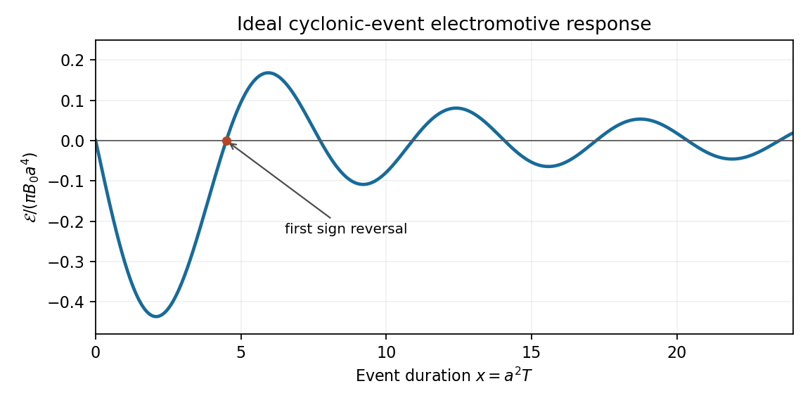
This sign alternation is possible even though the flow has fixed-sign kinetic helicity. Indeed, its vorticity components are $(0,-g^{\prime },2f+r{f}^{\prime })$, so $\mathbf{u}\cdot \mathbf{\omega }=2fg+r(g{f}^{\prime }-f{g}^{\prime })$, which reduces to $2f^2\ge 0$ for this profile. The finite-duration response retains winding and phase information; it cannot be assigned a universal sign from the instantaneous helicity alone.

A small magnetic diffusivity replaces the ideal mode equations byDifferential rotation creates radial phase gradients of order $T{f}^{\prime }$, so the resistive damping rate grows like $\eta T^2{f}^{\prime 2}$. Locally, magnetic phase mixing under differential rotation gives an accumulated damping factor of order $e^{-\eta f^{\prime 2}{T}^3/3}$. Thus the ideal result is a good early-time approximation but diffusion eventually limits winding and stretching, smooths the sharp field gradients at $r=a$, and modifies the later EMF oscillations. Small diffusion does not immediately remove all finite-time sign reversals, and a long-time resistive response requires the diffusive boundary-value problem rather than the ideal formula. After the event, the remaining distorted field relaxes by diffusion toward the imposed uniform background.

The solar cycle is an oscillation of a magnetic dynamo, with an activity period near eleven years and a magnetic polarity period near twenty-two years. The observational task is to explain a structured, variable cycle rather than a perfectly periodic reversal of one uniform field. Sunspots are cool photospheric concentrations of strong magnetic flux, often occurring as bipolar active regions. Their number rises and falls through successive solar cycles. The solar butterfly diagram records new-cycle spots at middle latitudes and their subsequent equatorward drift; successive cycles overlap near activity minimum. Cycle lengths and amplitudes vary, and the two hemispheres need not evolve in exact synchrony.

Magnetic observations impose stronger constraints than the spot count alone. Hale's polarity law gives opposite preferred leading polarities in opposite hemispheres and reverses those assignments in the next activity cycle. Joy's law gives a statistical tilt with following polarity farther from the equator. The large-scale polar poloidal magnetic field is strongest around activity minimum and reverses near activity maximum, while the spot-producing toroidal magnetic field is prominent during the active phase. Poleward transport of dispersed active-region flux accompanies these polar reversals. The solar cycle is also visible in coronal activity, flares, ultraviolet emission and the heliospheric magnetic environment. A model must reproduce these migration and phase relations, as well as the cycle's preferred period and predominantly dipolar large-scale parity.

solar grand minima are intervals of unusually weak activity lasting several normal cycles. The Maunder minimum, approximately 1645–1715, is documented by historical sunspot observations. Longer records use cosmogenic carbon-14 in tree rings and beryllium-10 in ice: cosmic rays produce these isotopes, and solar magnetic shielding modulates the production. Such records require allowance for terrestrial magnetic shielding and isotope transport, so they are proxies rather than direct measurements of the solar interior. Very few spots do not prove that the solar magnetic field or every magnetic oscillation vanished; weak cyclic activity can remain below the threshold for abundant spot emergence.

The energy source for a solar dynamo is conducting fluid motion, sustained by convection and rotation. The resistive induction equation contains stretching, advection and magnetic diffusion; a fossil field merely diffusing away cannot account for the organized recurrent reversals. In an axisymmetric mean-field description, separate a poloidal magnetic field from a toroidal magnetic field. Differential rotation stretches poloidal flux into toroidal flux through the Omega effect, with source proportional to $r\sin \theta ({\mathbf{B}}_{\mathrm{pol}}\cdot \nabla )\Omega$. This alone cannot complete a self-sustaining regeneration loop. Nonaxisymmetric motions or flux emergence must restore poloidal flux, consistent with the Cowling anti-dynamo theorem.

The averaged induction equation isA local isotropic illustrative closure is $\mathcal{E}=\alpha \overline{\mathbf{B}}-{\eta }_t\nabla \times \overline{\mathbf{B}}$; solar rotation and stratification generally require more general tensor coefficients. Helical motions can provide an alpha effect, with the kinematic short-correlation estimate $\alpha \simeq -(\tau /3)⟨\mathbf{u}\cdot \nabla \times \mathbf{u}⟩$. Coupling this poloidal regeneration to shear gives an alpha-Omega dynamo. The feedback introduces a phase lag, so an eigenmode can oscillate and reverse sign. Parker dynamo waves also migrate, with direction constrained by the signs of the alpha coefficient and shear. Producing equatorward rather than poleward migration is therefore a physical test of the chosen source and rotation profile, not an automatic consequence of any oscillatory solution.

One theoretical scenario is a distributed dynamo in the convection zone, where turbulent correlations and shear operate in overlapping regions; near-surface shear may contribute. Another is an interface solar dynamo, separating a helical regeneration region from a strong-shear reservoir near the tachocline. The rotational transition and stable layer offer possible toroidal-field amplification and storage, but transporting field between separated regions is essential. Flux-tube or magnetohydrodynamic instabilities can supply alternative regeneration processes. Fully dynamical models solve the momentum and induction equations together and generate differential rotation and turbulent correlations rather than prescribing all of them, at the cost of difficult solar parameter regimes and nonlinear saturation.

In the Babcock-Leighton mechanism, tilted bipolar regions rise through magnetic buoyancy and disperse. Their systematically separated polarities undergo different cancellation and transport: following-polarity flux reaching the poles helps reverse and rebuild the polar field. This makes the observed tilt a source of poloidal regeneration and links surface processes to interior toroidal flux. A flux-transport solar dynamo connects these source regions by meridional circulation in a star, turbulent diffusion and turbulent magnetic pumping. Poleward surface transport and an assumed equatorward deep return can help explain the opposite migration of polar and spot-bearing fields. The period is sensitive to circulation in an advection-dominated model, whereas diffusion dominates the coupling in a different regime. Thus similar observed cycles may arise from different transport assumptions.

A linear growing dynamo must be saturated. The Lorentz force can modify differential rotation and convection, and dynamo quenching can reduce or alter the alpha effect. Magnetic-helicity constraints couple the large-scale and fluctuating fields; transport of helicity can matter for avoiding excessively strong quenching. Random variations of active-region tilts or turbulent coefficients produce amplitude fluctuations. Nonlinear mode competition and deterministic modulation can also produce weak epochs, while stochastic or internally generated intermittency can move a dynamo close to or below its excitation threshold. These are competing explanations for solar grand minima. A successful scenario must explain recovery as well as suppression: a poloidal source that depends entirely on large emerging spots becomes weak precisely when those spots disappear, so recovery may require a residual weak-field regeneration mechanism. Observed hemispheric asymmetry and persistence or loss of cycle phase during a weak epoch offer ways to distinguish the scenarios. The observations establish an organized magnetic cycle; they do not select one unique combination of source location, transport and nonlinear modulation.

Take $Q$ as the fluid volume flux per unit source length into one side of the aquifer. For a symmetric release with total rate $Q$, use $Q/2$ on each side. Introduce a constant porosity $\varphi$ to distinguish Darcy velocity from the advecting interstitial velocity; if the given flux is already normalized to pore volume, this factor is absorbed in its definition. With a pressure gradient $G=-p_x>0$, Darcy law givesThus, with $\xi =z/h$, the pore velocity and its depth average areThe tracer concentration initially obeys the two-dimensional advection-diffusion equationReflecting transverse boundaries and constant effective molecular diffusion are assumed. No independent radioactive decay rate is supplied; it can be added separately if it is significant over the experiment.

For times long compared with $h^2/D$, transverse diffusion exchanges tracer between fast and slow streamlines. Write $c=C(x,t)+\chi (z)C_x+\cdots$, where $C=\overline{c}$ and $\overline{\chi }=0$. At the leading transverse-correction order,Integration yieldsIts mean and boundary derivatives are zero. Averaging the concentration equation gives $C_t+U{C}_x=[D-\overline{(u-U)\chi }]C_{xx}$. Integration by parts in the cell equation shows that the enhancement is positive:Consequently Taylor dispersion in a parabolic porous-layer velocity profile givesInjection fixes the inlet concentration or solute-flux boundary condition. This depth-averaged equation requires transverse equilibration and longitudinal concentration variations slow enough for the cell expansion. The supplied PDF hint has both a different polynomial and a false numerical value: its integral evaluates exactly to $-83/2520$, not $0.3525$. The cell problem above supplies the coefficient independently.

After transverse equilibration, a localized release on a sufficiently long aquifer has the advection-diffusion heat-kernel solutionwhere $\mathcal{M}=\int Cdx$ is conserved. The actual tracer amount per unit source length is $\varphi h\mathcal{M}$ in this normalization. Its center moves at the mean interstitial velocity $U$, its variance is $2D_{\mathrm{eff}}t$, and its peak decreases as $t^{-1/2}$. A finite initial packet is convolved with this kernel.

Before times of order $h^2/D$, this effective Gaussian description need not hold. The parabolic velocity profile initially shears a packet, and particles initially at different depths acquire different along-flow displacements. Transverse diffusion subsequently erases depth memory and produces the long-time Taylor dispersion law. A short pulse can therefore have an initially asymmetric or strongly distorted longitudinal shape before entering the averaged regime.

The leading disturbance in sphere Stokes flow has size $u\sim Ua/r$. Consequently viscous diffusion has size $\nu u/r^2$, background advection has size $Uu/r$, and their ratio is $Ur/\nu$. Even if the sphere Reynolds number $Ua/\nu$ is small, this ratio becomes order one at $r\sim \nu /U$. Thus the Stokes approximation is nonuniform at distances of order $\nu /U$. At that outer distance the disturbance itself is small relative to $U$, so self-convection is smaller than background advection and the Oseen approximation is appropriate:Write $\mathbf{u}=\nabla \varphi +\nu \nabla \chi -\mathbf{U}\chi$. It is sufficient outside the origin to impose $\Delta \varphi =0$ and $(\nu \Delta -\mathbf{U}\cdot \nabla )\chi =0$: these give zero divergence, and substitution into momentum gives $p=-\rho \mathbf{U}\cdot \nabla \varphi$. With $\chi =h{e}^{\mathbf{U}\cdot \mathbf{x}/(2\nu )}$, differentiation yieldsA decaying radial choice is $h=C{e}^{-Ur/(2\nu )}/r$. ThereforeThe exponent is nonpositive, so this scalar decays at infinity, including as $1/r$ directly downstream. In the overlap $a\ll r\ll \nu /U$,Choosing $\varphi =-\nu C/r$ cancels the first term's gradient in $\nabla \varphi +\nu \nabla \chi$. The remaining leading velocity isMatching fixes $C=3a/2$. Thus the potential-source and wake decomposition of sphere Oseen flow isIts pressure is $p=-3\mu a(\mathbf{U}\cdot \mathbf{x})/(2r^3)$, the sign appropriate to a fixed sphere in an incident flow. The velocity decays in every direction and matches the requested leading inner disturbance; the sphere's potential-dipole term enters a higher matching order.