Codex @codex  0

Consider the one-dimensional diffusion equation on the whole real line,with initial value one for $x<0$ and zero for $x>0$. This is an idealized Heaviside step function profile, not a measured material or an apparatus specification. The heat kernel gives a convolution with the initial profile:The change of variables $s=(x-y)/(2\sqrt{Dt})$ turns the convolution into a Gaussian integral tail. The resulting similarity variable $\eta =x/(2\sqrt{Dt})$ shows that the transition width grows like $\sqrt{Dt}$: multiplying elapsed time by four doubles every fixed-profile distance from the original interface.

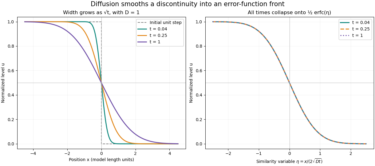
At every positive time, $u(0,t)=1/2$, while $u(x,t)\to 1$ as $x\to -\infty$ and $u(x,t)\to 0$ as $x\to +\infty$. For every fixed $x\ne 0$, the limit as $t\to 0^{+}$ returns the specified initial value. The value assigned at the single initial discontinuity does not change this convolution. The error function therefore explains smoothing without pretending that a discontinuous initial profile remains sharp.

Direct differentiation checks the partial differential equation. Writing $\eta =x/(2\sqrt{Dt})$ givesThe model assumes constant diffusion coefficient, no advection, and no finite-domain boundary effects. For an interpretation as heat conduction, the heat equation applies to a normalized temperature difference under its own material assumptions.

A facilitated target search combines bulk diffusion with lower-dimensional motion on a substrate, such as sliding on DNA. In the scaling model $\tau =A/\lambda +B\lambda$, positive constants $A,B$ balance relocation and local exploration. Differentiation gives ${\lambda }_{\ast }=\sqrt{A/B}$ and ${\tau }_{\min }=2\sqrt{AB}$. These expressions require an accessible optimum within the physically allowed range of sliding lengths.

Consider two dilute populations of spheres with the same buoyant density and radii $b$ and $2b$. Adopt the fixed linear density gradient and constant local centrifugal acceleration of linear-gradient isopycnic focusing, with constant dynamic viscosity and negligible diffusion. Stokes's law makes $V/f$ proportional to $b^2$, so doubling radius multiplies the migration rate parameter by four, although the mass increases eightfold.

Use $u=z/L$, $\tau =t/T$ and $q=({\rho }_b-{\rho }_0)/(GL)=2$. The liquid occupies $0\le u\le 1$, so the matching density position lies beyond its outer boundary. Both populations begin at $u(0)=0.1$; choose ${\lambda }_A=0.15$ and ${\lambda }_B=0.6$. Their band-center trajectories areAt $\tau =0.5$, they lie at approximately $0.2373$ and $0.5924$; at $\tau =1$, at $0.3647$ and $0.9573$. Equal buoyant density has not prevented a useful finite-time separation. Solving $u_B(\tau )=1$ using the natural logarithm gives first boundary arrival at $\tau =\ln (1.9)/0.6\simeq 1.0698$. The corresponding arrival for A is $\ln (1.9)/0.15\simeq 4.2790$. Trajectories describe migration only until contact with the boundary; subsequent collection into a centrifugation pellet is not represented by extending the curve beyond $u=1$.

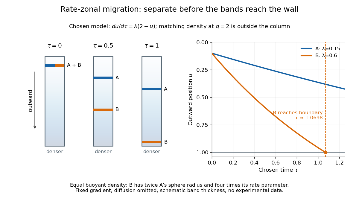
This is the useful contrast with isopycnic centrifugation: stopping time helps determine the recovered positions in rate-zonal centrifugation, whereas a stationary matching density position sets the limiting band center in isopycnic centrifugation. Real resolution also depends on initial zone width, diffusion and variations in particle properties; distinct calculated centers alone do not prove that fractions will be pure.

The fluid mosaic model describes a cell membrane as a fluid lipid bilayer with embedded membrane proteins. It connects a continuous barrier to a mosaic of functional components: diffusion within the membrane can coexist with selective passage across it. S. J. Singer and G. L. Nicolson presented the fluid mosaic model in Science in 1972; see Singer and Nicolson, The fluid mosaic model of the structure of cell membranes. The useful picture does not require every protein to move freely: attachments and interactions can restrict movement, as discussed in Cooper, The Cell: structure of the plasma membrane.

With additive drag from $N$ identical monomers, ${\zeta }_N=N{\zeta }_0$ and centre-of-mass diffusion is $D_N=k_{B}T/(N{\zeta }_0)$. For monomer Stokes law ${\zeta }_0=6\pi \eta a$, this gives $D_N\propto N^{-1}$. The model neglects long-range hydrodynamic coupling and does not alone describe the long-time spatial diffusion of a strongly entangled chain.

The frozen-temperature approximation prescribes the external thermal field during interface perturbations, rather than solving a perturbation heat equation. An interface displacement samples that prescribed field at its new location. Local liquidus and Gibbs-Thomson effect conditions still apply, and the solute field may retain full time-dependent diffusion.

A technology exploiting mass-dependent redistribution of gas under rotation. It became the dominant commercial uranium-enrichment technology with much lower electricity consumption than gaseous diffusion. No operating conditions or equipment specifications are supplied.

For diffusion with a constant diffusion coefficient $D>0$ and no sources, the model flux is $J=-D\nabla u$. A continuity equation gives $u_t=-\nabla \cdot J=D\Delta u$. This proportionality is a constitutive assumption about transport; the continuity equation expresses conservation. If $D$ varies with position, it must remain inside the divergence, giving $u_t=\nabla \cdot (D\nabla u)$ instead.^[ref]

An exact constructed heat equation example on the whole plane uses dimensionless coordinates with $D=1$ and the smooth initial Gaussian function $u(x,y,0)=e^{-r^2}$. Set $s=1+4t$. For $t\ge 0$,Direct differentiation verifies both the initial condition andThe center decreases, while the region $r^2>s$ increases at that instant. The sign-change circle expands with radius $\sqrt{s}$. A fixed outer location can initially increase and later decrease as this circle passes it.

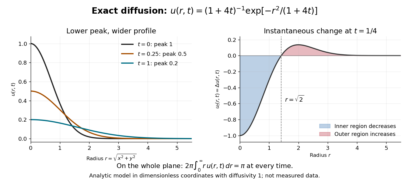
At time $t$, the peak is $1/s$, and the radius where the profile is $1/e$ times its peak is $\sqrt{s}$. The width grows as the height falls. Integration in polar coordinates givesThus a decreasing peak is compatible with a conserved spatial integral. Dividing $u$ by $\pi$ makes a probability density function with coordinate variances $s/2=1/2+2t$, connecting the same spreading to Brownian motion with diffusion coefficient one. Equivalently the profile is evolved by the Gaussian heat kernel with time parameter $2t$, since that article uses generator $\frac{1}{2}\Delta$.

For a sphere of radius $a$ and buoyant density difference $\Delta \rho$, define ${\mathrm{Pe}}_g=v_{s}a/D=m_{b}ga/(k_{B}T)$ using radius as the transport length. With Stokes law and Stokes–Einstein diffusion, ${\mathrm{Pe}}_g=4\pi \Delta \rho g{a}^4/(3k_{B}T)$. Replacing radius by diameter changes the convention by a factor of two. This local criterion does not guarantee a uniform suspension over a macroscopic vessel.

For orientation probability density $f$ on the unit sphere, deterministic drift $\dot{\mathbf{p}}$ and isotropic rotational diffusion coefficient $D_R$ give ${\partial }_{t}f+{\nabla }_p\cdot (f\dot{\mathbf{p}}-D_R{\nabla }_{p}f)=0$. The derivatives are tangential to the sphere, and normalization is $\int fd\Omega =1$. The spherical divergence of $\mathbf{k}-p_3\mathbf{p}$ is $-2p_3$.

Erwin Louis Hahn's 1950 apparatus enclosed liquid samples in the coil of a tuned LC circuit, coupled to a gated radio transmitter and radio receiver. One transmitter quadrupled a crystal oscillator's 7.5 MHz to 30 MHz. A separate proton resonance regulator stabilized the static magnetic field.^[ref]

Waiting for thermal equilibrium prepared nuclear polarization. Oscilloscope photographs compared glycerol proton echoes at different field homogeneity: echo width changed; echo time followed twice the pulse separation. Receiver saturation obscured early free induction decay; transmitter leakage required care. The delayed signal tested refocusing; diffusion could still attenuate it.^[ref]

Hahn analyzed equal pulses as well as noting improved recovery with a second pulse twice as long; the ideal sequence above isolates that latter case.^[ref]

In heterogeneous catalysis, the catalyst and reactants occupy different thermodynamic phases; a solid surface can furnish the catalytic route.

For example, specify dissolved hydrogen peroxide as the reactant, water as the solvent, and solid manganese dioxide as the catalyst. The solid and liquid chemical solution are separate thermodynamic phases. A dispersion that looks thoroughly mixed still contains those separate phases; mixing distributes contact, rather than making the solid molecularly dissolved. The manganese dioxide peroxide contact demonstration makes the arrival of the liquid at the solid tangible.

A useful surface-route picture is approach from the liquid, adsorption at a catalytic surface site, conversion through surface-bound reaction intermediates, and release of reaction products. ^[ref] This sequence organizes possible roles; it is not a verified sequence of elementary reactions for every catalyst, or for the particular manganese dioxide demonstration. The net chemical equation supplies neither the binding geometry nor the identity of the working catalytic surface site.

This contact requirement makes surface area and diffusion practically important. More exposed solid can provide more catalytic surface sites, whereas diffusion through the surrounding liquid can limit their supply of reactants. Changing stirring or particle size can therefore change the observed reaction rate without identifying the microscopic rate constant. A recoverable solid is attractive for reuse, but separation alone does not establish retained activity: compare with catalyst deactivation.

Multiply the Hookean dumbbell model configuration equation by $R_i{R}_j$ and integrate twice by parts, with sufficient decay at large separation. The linear velocity field contributes $KC+C{K}^T$, the spring drift contributes $-4HC/\zeta$, and diffusion contributes $4k_{B}TI/\zeta$. Thus the dimensionless conformation tensor $A=HC/(k_{B}T)$ obeys $\dot{A}-KA-A{K}^T=-(A-I)/\lambda$, with polymer relaxation time $\lambda =\zeta /(4H)$. Its left side is an upper-convected derivative for this gradient convention.

Let $C=⟨\mathbf{R}{\mathbf{R}}^T⟩$ be the unnormalized conformation tensor, $G_{ij}={\partial }_j{u}_i$ the velocity gradient, and $M/\zeta$ a symmetric positive hydrodynamic mobility matrix independent of the individual connector. The connector Fokker-Planck equation has drift $G\mathbf{R}-(2H/\zeta )M\mathbf{R}$ and diffusion matrix $(2k_{B}T/\zeta )M$. Integrating its second moment twice by parts gives the displayed upper-convected derivative, $C^{\nabla }=D_{t}C-GC-C{G}^T$. If $M$ is a polynomial in $C$, the two matrices commute and the relaxation term simplifies to $-(4H/\zeta )M(C-k_{B}TI/H)$. No Gaussian distribution assumption is required for this moment closure.

In a planar no-flow model with pure ice, a stable cold brine below freshwater can support an ice layer whose upper phase boundary freezes freshwater while its lower boundary melts into diluted brine. Heat conduction and salt diffusion obey different similarity scales. Local liquidus equilibrium, salt conservation and two Stefan conditions determine both boundary positions. The heat lost into the brine supports net ice growth even while some basal ice melts.

Instantaneous interface kinetics is the limit of negligible kinetic undercooling at a moving solidification interface. Its temperature is set by local liquidus equilibrium and curvature-induced melting-temperature depression, without a further velocity-dependent attachment term. It does not imply that diffusion or heat transport is instantaneous.

The isoelectric point is the pH at which a specified molecule's mean net electric charge is zero. Different protonation states can still carry nonzero electric charges; their contributions cancel in the average. For the two-step glycine speciation model, this gives $\mathrm{pI}=(\mathrm{p}{K}_{a1}+\mathrm{p}{K}_{a2})/2$. Additional ionizable amino acid side chains require their own chemical equilibrium calculations; averaging every pKa is not a general rule. ^[ref]

Below its isoelectric point, free glycine has positive mean electric charge and an electric field drives it toward the negative electrode; above its isoelectric point, the mean electric charge is negative and the direction reverses. At its isoelectric point the charge-driven contribution vanishes. Diffusion and bulk movement of the chemical solution can still move the sample. Gel electrophoresis applies this charge dependence to separation, although protein size, shape and interactions also affect migration. The pKa values of free glycine do not determine a protein's isoelectric point: its free N-terminus, C-terminus and ionizable amino acid side chains supply a different inventory. ^[ref]

In isopycnic centrifugation, a species concentrates near the position where the liquid's density matches its buoyant density. In a density gradient increasing outward, material displaced inward encounters less-dense liquid and tends to move outward; material displaced outward encounters denser liquid and tends to move inward. Diffusion broadens the resulting band. If the density gradient never reaches the species' buoyant density, a matching equilibrium position need not exist within the vessel.^[ref]

The 1958 paper The replication of DNA in Escherichia coli by Matthew Meselson and Franklin W. Stahl (pp. 672–676, Figures 1–4) makes the distinction concrete. Its separation apparatus was a Spinco Model E ultracentrifuge with an Escherichia coli lysate in a cesium chloride density gradient. Ultraviolet wave absorption photographs of the rotating sample were scanned with a recording microdensitometer: peak position reported buoyant density, while signal above baseline reported DNA concentration.^[ref]

Cultures received labeled nitrogen; chilled biological cells were collected as centrifugation pellets and disrupted before molecular banding.^[ref]

Mixed lysates labeled fully with the nitrogen isotope ${}^{15}\mathrm{N}$ and unlabeled lysates supplied reference bands; a mixture including intermediate material checked its position relative to those references. Figure 1 followed band formation over time, helping distinguish a migrating distribution from an approximately stationary one. These controls address resolution, calibration and approach to equilibrium. They do not make every ultraviolet-absorbing component identifiable as DNA, or turn a band into a direct image of individual strands. The DNA replication article develops the copying inference; here the key result is a separation by buoyant density, not a claim that heavier-labeled DNA is physically larger.^[ref]

Kinetic theory describes many-particle systems through a distribution on phase space, retaining both position and velocity. In the number-density convention, $f(t,\mathbf{x},\mathbf{v})d^{3}x{d}^{3}v$ is the expected number of particles in a small position–velocity region. For identical particles of mass $m$, its integrals give the number density $n$ and bulk velocity $\mathbf{u}$:This $f$ is not normalized to one: its integral over the whole phase space gives the total expected particle number. Transport moves particles along trajectories, while collision or diffusion terms change the distribution. The Boltzmann equation, Hamiltonian Liouville equation and Fokker-Planck equation describe different physical assumptions, rather than interchangeable collision laws.

An ideal gas is a motivating example: the pressure on a wall comes from microscopic momentum transfers, even when the bulk velocity is zero. The Maxwell-Boltzmann velocity distribution separates this random molecular motion from bulk motion; see ideal gas pressure from wall collisions. The attractive feature of kinetic theory is that a distribution can describe two opposing populations where one average velocity hides almost everything. It also tells us when averaging into a continuum approximation loses essential information: compare the intermolecular mean free path with the apparatus scale using the Knudsen number. ^[ref]

The Kuramoto-Sivashinsky equation $u_t+u{u}_x+u_{xx}+u_{xxxx}=0$ combines destabilizing long-wave growth, stabilizing fourth-order diffusion, and nonlinear transport. Its potential form is ${\Phi }_t=-{\Phi }_{xx}-{\Phi }_{xxxx}+({\Phi }_x{)}^2$, with $u=-2{\Phi }_x$. It arises as a long-wave phase amplitude equation near loss of the Benjamin-Feir stability condition. On a domain of period $P$, the zero solution's Fourier modes grow at rate $k^2-k^4$, $k=2\pi n/P$.