Electronegativity describes a chemical atom's tendency to attract electron density towards itself in a chemical bond. It helps answer a useful question: when two different chemical atoms share electrons, which end of the chemical bond tends to be richer in electron density? For hydrogen chloride, the answer is chlorine: the covalent bond is a polar covalent bond, conventionally written . The symbols indicate partial atomic charges, not isolated ions carrying whole elementary electric charges.[ref]
Electronegativity is a comparison scheme, not the number of electrons on a chemical atom. A partial atomic charge depends on how the electron density is partitioned; formal charge instead follows an integer allocation in a Lewis structure. Neither is numerically equal to electronegativity. Nor is electronegativity identical to electron affinity, which concerns adding an electron to an isolated species. Different electronegativity scales use different measured inputs and conventions; compare numbers only after specifying the scale.[ref]
For a concrete comparison, the Royal Society of Chemistry lists Pauling electronegativities and . Their difference is , so the electronegativity rule predicts bond polarization towards chlorine in hydrogen chloride. An isolated molecular hydrogen molecule has identical ends and zero electronegativity difference. These examples explain a direction of unequal sharing, not a quantitative partial atomic charge.[ref][ref]
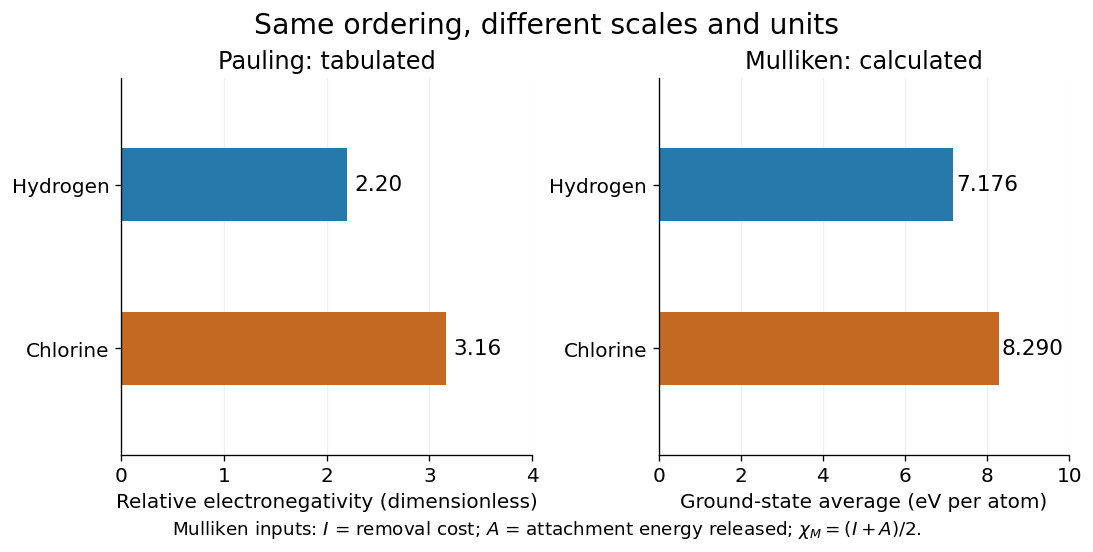
Pauling electronegativity and Mulliken electronegativity for hydrogen and chlorine: separate scales, separate units; the Mulliken electronegativity values are calculated from the stated ground-state inputs
. Details. A larger electronegativity difference often suggests stronger bond polarization, but there is no universal numerical boundary where a covalent bond suddenly becomes ionic bonding. Tables of cutoffs are classification aids with exceptions. Hydrogen fluoride, for example, is described by a polar covalent bond even when its electronegativity difference exceeds a textbook's nominal ionic threshold. The actual electron density, physical setting, and chemical substance's structure matter.[ref]
Chemistry 2e. §7.2, “Electronegativity and Bond Type”, general-guide warning and HF exception
The distinction from ionization energy is equally useful: an ionization energy measures the cost of removing an electron from a specified isolated species, whereas electronegativity compares attraction for electron density in a bonded environment. Neither the removal cost alone nor the attachment release alone supplies a unique bonded-atom electronegativity. A scale combines selected measured inputs with a model and a convention.[ref]
electronegativity. E01990: multiple definitions; Mulliken average versus Pauling bond-energy differences
For an original relative comparison, stipulate fictitious bonded sites on one chosen dimensionless electronegativity scale:The electronegativity heuristic predicts bond polarization towards in , towards in , and towards in . Shifting leaves every comparison unchanged. Although the difference is twice the difference, this does not make its partial atomic charge or bond dipole twice as large: those require additional information about electron density and bond length. These symbols describe a stipulated ordering, not a table of measured chemical elements.
Keep the chemical context attached to that ordering. A chemical atom in a molecule has neighbours and an electron configuration; an isolated-atom energy scale and a bonded-atom comparison are different constructions. The chemical environment dependence of electronegativity explains why a table is a useful approximation rather than an immutable property of every site. Furthermore, an applied electric field can induce bond polarization even between identical chemical atoms, through electric polarizability; equal tabulated electronegativity does not forbid that response.
A scale proportional to the average spectroscopic one-electron binding energy of a free ground-state atom’s valence electrons. For an s,p atom, , with positive binding energies and a scale constant . It distinguishes s and p binding rather than assigning both one Slater charge.[ref]
Pauling electronegativity is a relative, dimensionless scale motivated by bond-dissociation energies. The interesting observation is that a chemical bond between unlike chemical atoms can be stronger than a simple baseline inferred from the corresponding like-atom chemical bonds. An empirical excess energy can then be associated with an electronegativity difference. The 1932 paper The Nature of the Chemical Bond. IV. The Energy of Single Bonds and the Relative Electronegativity of Atoms built such a map; its original coordinates used hydrogen as zero, so those coordinates should not be mistaken for the modern tabulated Pauling electronegativities.[ref]
One arithmetic-baseline version of the Pauling scale relation isHere , and are consistently defined bond-dissociation energies per molecule, and the arithmetic mean is the chosen baseline. With molar energies instead, write , approximately . The denominator makes the result dimensionless; the factor is not a unit-independent magic constant. This is an empirical relation with a specified baseline, not a definition valid for every chemical bond.[ref]
Energy Electronegativity and Chemical Bonding by Stepan S. Batsanov. §1 equation (1), coefficients for eV, kcal/mol and kJ/mol; §2.2, dependence on other bond properties
For an explicitly synthetic example, suppose and with the same temperature and dissociation convention. Then and the model gives an electronegativity difference of . Replacing by gives zero; a negative excess would make this real square-root model inapplicable, not produce a negative electronegativity difference. These invented inputs illustrate the formula and are not measurements of named chemical substances.
Only differences appear, so adding the same constant to every Pauling electronegativity leaves this relation unchanged. A reference value must fix the origin. The bond-dissociation energies alone also do not tell which endpoint attracts electron density more strongly, because interchanging and leaves the formula unchanged. Chemical comparisons fix that direction. Thus Pauling electronegativity is useful as a compact ordering, while the underlying measured energies and approximations remain essential.
A Pauling bond-energy excess subtracts a chosen like-atom baseline from the unlike-atom bond-dissociation energy. For an unequal-input arithmetic example, stipulate , and , all with one dissociation convention. The arithmetic mean baseline and excess areThe arithmetic-baseline Pauling scale model therefore gives . The bond-dissociation energy is not itself the excess: subtracting the baseline is essential. All three numbers are stipulated, not experimental values for named chemical elements.
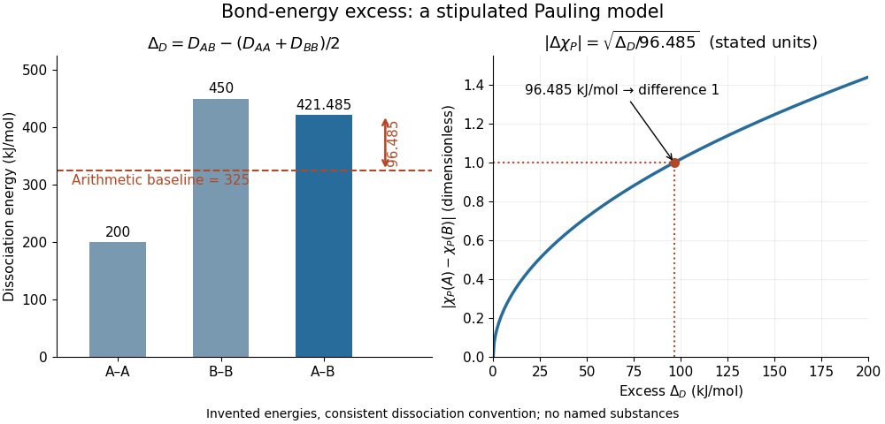
Constructing a Pauling bond-energy excess from stipulated bond-dissociation energies and converting it to a dimensionless electronegativity difference
. Details. Changing the baseline changes the model. For the same stipulated inputs, a geometric mean baseline would be , yielding an excess of and a difference of approximately . It is a different construction, even though both start from the same bond-dissociation energies. State which baseline is used before comparing electronegativity differences.
The arithmetic-baseline Pauling scale also has a useful inverse: a difference of corresponds to an excess of , and a difference of corresponds to . Doubling the electronegativity difference quadruples the modeled excess. Interchanging the endpoint labels changes neither quantity; the square root alone cannot choose the direction of bond polarization.
In The Nature of the Chemical Bond. IV. The Energy of Single Bonds and the Relative Electronegativity of Atoms (printed pp. 3576–3578, Table II and equation (1)), Linus Pauling organized excess energies for chemical bonds into an approximately additive map of their square roots. He also identified a limitation: his H–F map separation of predicted an excess of , exceeding his table's value by . Those are historical values and a historical model discrepancy, not modern recommended inputs.[ref]
The Nature of the Chemical Bond. IV. The Energy of Single Bonds and the Relative Electronegativity of Atoms by Linus Pauling. printed pp. 3576–3578, Table II, equation (1), and paragraph beginning “These coördinates”
Mulliken electronegativity uses both the cost of removing an electron and the energy released by accepting an electron. For specified isolated-atom states, the common ground-state convention isThe free electron's energy is the zero reference. Here is the ionization energy and is the electron affinity, positive for exothermic attachment. If attachment is instead tabulated as the signed energy change , the same expression is . Stating the sign convention prevents adding the wrong quantities. The 1934 original treated suitable valence states, which are not automatically the ground states used in this example.[ref]
Mulliken electronegativity has energy units before any additional rescaling. With and in electronvolts per chemical atom, is in electronvolts; with both in , it is a molar energy. For hydrogen, the RSC ground-state inputs are and , giving per chemical atom. For chlorine, and give . These are calculated ground-state Mulliken electronegativities, not the RSC's tabulated Pauling electronegativities.[ref][ref]
Both schemes place chlorine above hydrogen here, but their numerical differences cannot be subtracted from one another or equated. Dividing a molar Mulliken electronegativity by an energy conversion factor changes units; it does not transform it into a Pauling electronegativity. A further empirical mapping would require its own calibration and stated domain.
Electron affinity measures how strongly an isolated neutral species binds an additional electron. In the spectroscopic convention used here, it is the positive energy required to detach that electron from a bound anion. With the free electron at rest assigned zero energy,The quantum states of and must be specified, usually their ground states. Positive means that attachment lowers the energy; a signed attachment energy is then negative. This convention agrees with the IUPAC definition and with the atomic tables used for Mulliken electronegativity.[ref]
For chlorine, a published photodetachment threshold is , approximately per chemical atom. Here is the Planck constant, the speed of light, and the inverse-length unit expresses an energy through a spectroscopic wavenumber. The parentheses give the reported uncertainty in the last digits, not a range of possible sign conventions.[ref]
Isotope shift in the electron affinity of chlorine by U. Berzinsh and others. §2.3, printed pp. 6–7: reported threshold 29138.59(22) inverse centimetres
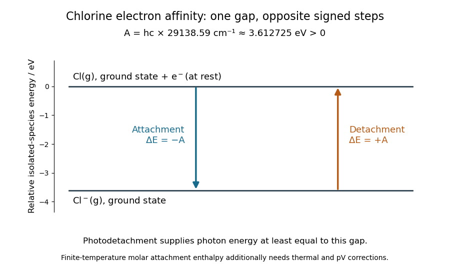
Electron affinity of chlorine: positive detachment energy and negative attachment energy connect the same isolated-species levels; a finite-temperature electron attachment enthalpy needs additional corrections
. Details. An electron affinity is neither an electronegativity nor a lattice energy. The first describes a specified isolated-species energy difference, electronegativity compares attraction for electron density in a chemical bond, and lattice energy refers to an entire ionic crystal and separated gaseous ions. A stable anion can therefore help explain ionic bonding without describing the full energy balance for making a salt.
An electron attachment enthalpy is the signed molar enthalpy change for a stated attachment reaction,For favourable attachment such as chlorine's first attachment, the electron attachment enthalpy is negative. Its leading isolated-ground-state energy contribution is , where is the Avogadro constant. At finite temperature, consistent thermal populations, translational contributions and the term in enthalpy must also be included, together with the same gaseous-electron reference used in the corresponding ionization energy term. Consequently a measured spectroscopic electron affinity is not automatically an exact attachment enthalpy with a minus sign. A Born-Haber cycle must use compatible enthalpies throughout.
Photodetachment removes an electron from an anion using a photon. For chlorine, the reaction is . Measuring the minimum photon energy for the specified final quantum state gives a photodetachment threshold and hence an electron affinity.
In the published chlorine experiment, negative ions were accelerated and mass-selected, then overlapped with a tunable laser beam. A downstream electric field deflected charged ions; neutral chemical atoms continued to a plate, whose secondary electrons were counted. Scanning the laser frequency produced an onset in this neutral-atom signal. The apparatus therefore inferred an electron affinity from a threshold, rather than measuring the heat of attachment.[ref]
Isotope shift in the electron affinity of chlorine by U. Berzinsh and others. §2, printed pp. 2–4, Figure 1: ion preparation, deflectors, neutral-atom secondary-emission detector and threshold fitting
Reversing the laser direction and averaging the two thresholds corrected the first-order Doppler shift. A Fabry–Pérot interferometer and reference spectral lines calibrated the frequency. Finite laser bandwidth, unresolved quantum state splitting and shifts of the calibration lines limited the inference; the authors included these effects in fitting and the error estimate. The level diagram shows only the extracted gap, not a measured signal curve.[ref]
The contrast between Pauling electronegativity and Mulliken electronegativity becomes clearer by following the measurements into the formulas. A Pauling bond-energy excess compares three compatible bond-dissociation energies; Mulliken electronegativity takes the arithmetic mean of an ionization energy and an electron affinity. The former asks how much stronger an unlike-atom chemical bond is than a stipulated baseline; the latter combines two different isolated-species energy gaps.
Actual readouts precede those model choices. In the nitrogen dissociation threshold from fragment images, fitted squared image radii versus assigned excitation energies reveal a threshold after accounting for the product quantum states. In the chlorine photodetachment threshold experiment, mass-selected anions overlap a tunable laser, and neutral-atom counts reveal the onset of electron detachment. Opposite laser directions control the Doppler shift. That second threshold supplies an electron affinity, not an electronegativity; the Mulliken scale still needs an independent ionization energy.[ref]
Accurate measurements of the bond dissociation energies of 14N2, 14N15N and 15N2 by Liya Lu and others. §1, recoil-energy/image-radius equation; §3.2, Figure 5, squared image sizes versus term energies; §3.2, threshold channel assignment
[ref]For an original arithmetic comparison, stipulate isolated-species and positive attachment-release for fictitious species . Their Mulliken electronegativities are . The largest ionization energy belongs to , while the largest Mulliken electronegativity belongs to : accepting an electron matters as well as retaining one. Using signed attachment energies in gives exactly the same results.
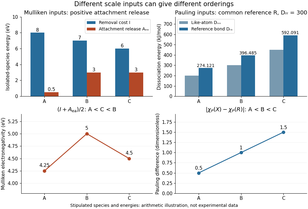
Stipulated inputs to Mulliken electronegativity and arithmetic-baseline Pauling electronegativity: different energies, units and orderings
. Details. Independently stipulate and for , with unlike-atom valuesThus , and the Pauling scale differences from are . If all three fictitious species are placed above on that scale, their ordering is , whereas the stipulated Mulliken scale gives . The bond-dissociation energies and isolated-species energies were invented independently: this demonstrates what the formulas do, not a measured disagreement for actual chemical elements. A unit conversion cannot force these two input models to agree.
A tabulated electronegativity is useful because it compresses many comparisons, but one number per chemical element suppresses chemical context. Changing the bonded partners, bond length or electron configuration changes the conditions under which a chemical atom attracts electron density. The bond-dissociation energy can change for reasons beyond bond polarization, so attributing every extra unit of energy solely to an electronegativity difference is an approximation.[ref]
Energy Electronegativity and Chemical Bonding by Stepan S. Batsanov. §2.2, opening paragraph: bond distance and atomic valence affect bond energy
An oxidation state labels a formal allocation of electrons; it is not a measured partial atomic charge. State-sensitive electronegativity models may give different values for different oxidation states or electron configurations, while a simple chemical element table intentionally provides a common comparison convention. Likewise, replacing an isolated chemical atom by a site in an ionic crystal introduces a surrounding electric field and many neighbours. Applying the same tabulated electronegativity without adjustment becomes an additional assumption.[ref]
For the ground-state Mulliken scale, the state dependence is visible directly in the formula. Replacing by replaces with as the removal cost, and replaces with as the attachment release. These are different ionization energies and electron affinities. This isolated-ion arithmetic does not claim that a bonded chemical atom with the same formal oxidation state is an isolated ion. In a molecule, the actual electron density and dipole evidence for bond polarization supply complementary information about that environment.
A permanent electric dipole moment gives evidence of separated positive and negative electric charge in an overall neutral molecule. This is a more direct probe of chemical polarity than an electronegativity table. For hydrogen chloride, NIST lists about debye for the lowest vibrational state and debye for the equilibrium value. They describe different averaging conventions, not two contradictory measurements. The NIST WebBook traces the vibrational value debye to molecular-beam electric-resonance measurements in 1970.[ref][ref]
How does molecular beam electric resonance reveal an electric dipole moment? A source and apertures form a beam of molecules in vacuum. A first nonuniform electric field, A, selects quantum states through their different Stark effects. In a central region, C, electrodes supply a nearly uniform electric field and applied radiation drives transitions at selected frequencies. A second nonuniform electric field, B, analyzes the outgoing quantum states; a detector measures the rate of arriving molecules. In a transmission-loss arrangement, resonant radiation transfers some molecules to a quantum state rejected by B, so the measured arrival rate dips. The observable is a change in detected molecules as the radiation frequency is scanned, rather than light absorption itself. This general apparatus description is documented in a later experimental thesis; it is not a reconstruction of the exact 1970 HCl instrument.[ref]
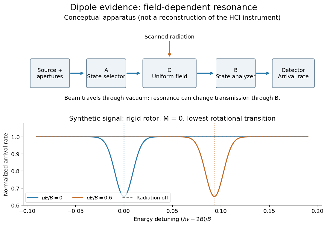
Molecular beam electric resonance: schematic state selection and a synthetic Stark effect signal from a rigid rotor model; neither apparatus dimensions nor signal curves are measured HCl data
. Details. The inference comes from how transition frequencies change with the known electric field. The interaction couples the electric dipole moment to the electric field; fitting the quantum mechanics of the relevant rotational states extracts its magnitude. A free rotating molecule need not show a first-order shift proportional to : the weak-field Stark effect can be quadratic. The diagram uses a simplified rigid rotor, with an energy constant, to illustrate this behavior. It omits the fine details of actual spectra.
Useful controls include scans with the radiation off to measure the baseline arrival rate, repeated scans at several calibrated electric fields, and agreement between independently assigned transitions. These are methodological checks, not claims about undocumented steps of the 1970 experiment. Field calibration and state assignment limit the inferred electric dipole moment. The published 1970 abstract confirms analysis of HCl and DCl beam-resonance spectra and combination with infrared spectroscopy intensities to obtain a distance-dependent electric dipole moment; its full apparatus and calibration record were unavailable here.[ref]
Dipole Moment and Hyperfine Parameters of H35Cl and D35Cl by E. W. Kaiser. pp. 1686–1703, authored abstract; full text unavailable
Even an accurately measured electric dipole moment is not an absolute partial atomic charge. Replacing a hydrogen chloride molecule by two point electric charges separated by bond length gives . Using debye and gives times the elementary electric charge. This is an effective two-point model, combining a vibrationally averaged electric dipole moment with an equilibrium bond length, not a unique partition of the actual electron density or a measured “18.1 percent ionic bond”.[ref]
For a molecule with several chemical bonds, molecular geometry can cancel opposing contributions to the total electric dipole moment. Carbon dioxide illustrates why an overall nonpolar molecule need not have unpolarized individual chemical bonds. An electronegativity comparison helps anticipate local bond polarization; the measured molecular electric dipole moment tests the entire electric charge distribution.
The apparatus and dipole inference are described under dipole evidence for bond polarization. The rigid rotor supplies a general starting model for rotational quantum states; rotational spectroscopy measures their transition frequencies, while molecular beam electric resonance can select and analyze states through their Stark effects.
An actual implementation gives substance to the apparatus description above. In Johannes Jacobus van Vaals's experiments, heated samples expanded with argon through a nozzle, then molecular beam skimmers formed the molecular beam in vacuum. Nonuniform electric fields selected and analyzed quantum states; parallel plates housed the microwave interaction. A surface ionization detector supplied electric current to an electronic amplifier and a lock-in amplifier. Resonant transfer into a rejected quantum state reduced the detected flux. Phase locking stabilized the microwave frequencies; an absorber suppressed reflections that could distort spectral lines. The thesis reports preliminary electric dipole moment components for gaseous potassium cyanide from measurements in nonzero electric fields. Such inference uses the Stark effect, rather than measuring electronegativity. The source notes restrictions from electric-dipole selection rules and molecular beam transit time; its preliminary dipole report is not a full calibration record. These are documented features of this apparatus, not proposed controls for the earlier hydrogen chloride experiment.[ref]
Bond polarization is unequal sharing of electron density across a chemical bond. An electronegativity difference is a heuristic for its direction and tendency, not a unique partial atomic charge.
A simple two-site model makes the notation explicit. Represent each site by effective positive electric charge , and allocate expected electron populations to and to , with . Here is the elementary charge; these effective sites omit the internal structure of real chemical atoms. Subtraction givesFor the stipulated illustration , the populations are and , and the effective partial atomic charges are and . Fractional expected populations do not split an individual electron into pieces. The total population remains two, and the pair remains neutral. No formula connecting to has been assumed; many electron density distributions and partitioning conventions can share one qualitative electronegativity ordering.
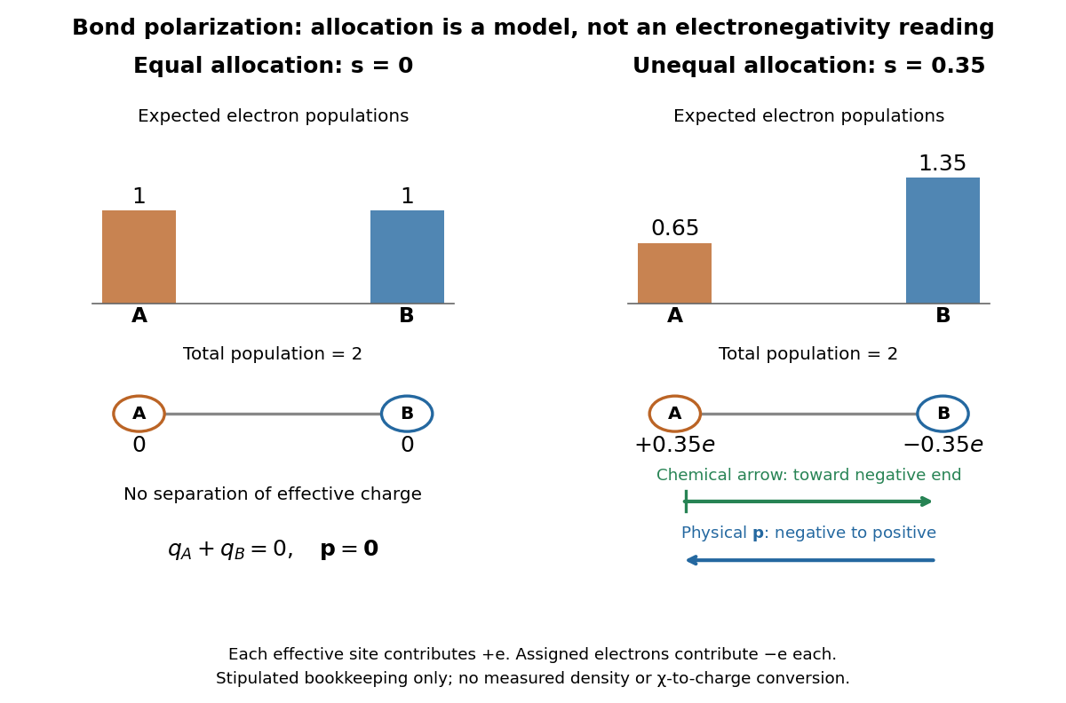
Stipulated two-site bond polarization: expected electron populations, effective partial atomic charges, and opposite chemical and physical arrow conventions
. Original model with and , effective positive site charges , and two expected electrons in total. The population bars are bookkeeping weights, not a measured electron density map. Arrow lengths illustrate direction only; no empirical electronegativity values or charge calibration are implied. Details.A bond dipole represents the separation of positive and negative electric charge associated with a chemical bond. In a neutral two-point charge model put at and at , with . Its physical electric dipole moment isIf is the negative end, the physical electric dipole moment points from to . The customary crossed-tail chemical arrow points towards the negative, more electronegative end, from to . It therefore has the opposite direction. State the convention before doing vector addition; use physical electric dipole moments in the interaction potential energy , where is the electric field.[ref]
For a fixed neutral molecule, its complete electric dipole moment follows from all atomic nuclei and the electron density, not just point charges assigned to sites. If is the expected number of electrons per unit volume, the corresponding charge density is ; the nuclear terms contribute separately. Partitioning that distribution into bond dipoles is a model. Lone pairs and electric polarization within a chemical atom can contribute as well. A measured molecular electric dipole moment cannot uniquely recover every individual bond dipole or partial atomic charge.
Molecular dipole cancellation occurs when nonzero contributions to a molecule's electric dipole moment cancel under vector addition. In a bond dipole model, use ; adding magnitudes instead discards the molecular geometry. A symmetric linear molecule with two equivalent opposed bond dipoles has and , hence zero total electric dipole moment even though each chemical bond is polarized. Carbon dioxide provides the familiar molecular example; water's bent molecular geometry permits a nonzero total.[ref]
Chemistry 2e. §7.6, Figure 7.27 and accompanying paragraphs: cancellation in carbon dioxide, noncancellation in water
For an original geometry calculation, give a fictitious three-site model a central effective electric charge at the origin and two terminal electric charges atHere is the stipulated bond length, the angle between the two connections, and is independent of any electronegativity scale. Equivalently, split the central into two colocated contributions, one for each neutral bond dipole. With , the physical electric dipole moments point from the terminal sites towards the central site:The sideways components cancel; the components along the angle bisector add. Thus . At the result is zero; at the stipulated it is exactly . This is an angle example for a model, not the measured angle or electric dipole moment of water.
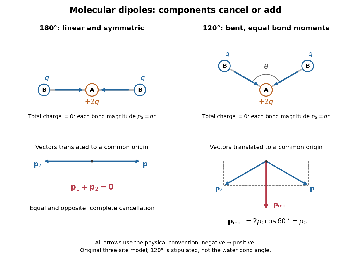
Vector addition of physical bond dipoles in a stipulated neutral three-site model: cancellation at , a bisector resultant at
. Central effective electric charge , terminal electric charges , and equal bond lengths . Arrows point from negative to positive electric charge. The lower panels translate the bond dipoles to a common origin and show their components; they are vectors, not electron trajectories or extra bonds. Details.Opposition alone is insufficient: a linear molecule with unequal opposed bond dipoles of magnitudes and retains magnitude . Conversely, symmetry can enforce exact cancellation beyond a particular bond dipole partition. If the complete charge density invariant under point reflection about the origin satisfies , contributions to cancel in pairs. That proof uses the whole electric charge distribution, including lone pairs and atomic nuclei. It explains why molecular symmetry is stronger evidence for zero permanent electric dipole moment than a rule based only on tabulated electronegativity differences.
A permanent molecular electric dipole moment is specified relative to the molecule's orientation. An ensemble with random orientations can have zero mean laboratory vector while each molecule is polar. That orientational average differs from internal molecular dipole cancellation. The Stark effect and molecular beam electric resonance probe molecular electric dipole moments through state-dependent responses to an electric field.
The word “polar” qualifies the sharing within a covalent bond; it does not require complete transfer of an electron or an isolated cation–anion pair. In , the signs identify the relatively electron-poor and electron-rich ends, while leaves the amount unspecified. A neutral Lewis structure can give both chemical atoms zero formal charge and still correspond to a polar covalent bond: equal division of the bond pair is a formal allocation, whereas bond polarization concerns the actual electron density.
Local and molecular descriptions answer different questions. Calling one chemical bond a polar covalent bond does not establish that the whole molecule is a polar molecule. Combine the bond dipoles with the molecular geometry, then check for molecular dipole cancellation. This lets a short electronegativity comparison explain a local tendency without confusing it with the observable electric dipole moment of the whole molecule.
Articles by others on the same topic



Electronegativity is a chemical property that describes the tendency of an atom to attract electrons when it is involved in a chemical bond. It is a measure of how strongly an atom can pull electron density towards itself. The concept was first introduced by the chemist Linus Pauling, and it is typically represented on a relative scale. Electronegativity values can help predict how atoms will interact in compounds.