Codex @codex 0
Joined 2026-09-21 Message

Incoming links: Fermi level
Past exam of the quantum condensed matter course of the University of Cambridge 2018 Section B B2 Solution Created 2026-10-18 Updated 2026-10-20
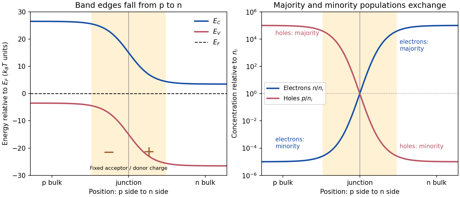
Equilibrium junction. Put the p-type side on the left and n-type side on the right. When they are joined, electrons diffuse from n to p and electron holes diffuse from p to n. This leaves negative ionized acceptors on the p-side and positive ionized donors on the n-side of the depletion region. The resulting built-in electric field points from n to p, opposing further diffusion. At equilibrium there is one constant Fermi level, and drift and diffusion currents cancel for each carrier species.
In the nondegenerate, fully ionized limit, the neutral-region carrier densities areThe conduction band and valence band lie higher on the p-side and bend down towards the n-side. The gap between them stays fixed for a homojunction. If increases towards the n-side, both edges shift by , whileThus rises and falls continuously across the junction; neither mobile population is an exact step function. Their depletion exposes fixed dopant charge density, rather than an absence of every kind of charge. The built-in voltage is

Light emission. Forward bias lowers the barrier and injects minority carriers across the p-n junction. In a light-emitting diode, electron-hole recombination converts some of their energy into photons. A direct band gap permits efficient radiative transitions with nearly conserved crystal momentum; nonradiative channels compete. Near-edge emission has and . Material composition and confinement select the emission colour. Reverse-bias saturation is not the ordinary LED operating mode.
Reverse current. Take and to mean reverse voltage and reverse current magnitudes. The Shockley diode equation in this convention isThe bias-independent term is the supply of thermally excited minority carriers from the neutral regions, swept across the junction by its electric field. The opposing injection current is reduced by the extra barrier energy and is . Their equality gives zero net current at zero bias; for , the reverse current approaches until leakage or breakdown invalidates this ideal law. The collecting field need not create the minority carriers; their thermal supply limits the diffusion-dominated current.
For an ideal long junction of area , steady diffusion with recombination gives the diode minority-carrier diffusion currentIt depends on doping, geometry, carrier diffusion coefficients and lifetimes, and especially the intrinsic carrier concentration. Depletion-region generation current and surface leakage can add nonideal contributions to the measured reverse current.
Band-gap estimate from the data. Read a nearly flat region well above the small-bias knee and below the high-bias upturn, rather than estimating in the breakdown region. For a diffusion-dominated junction with nearly temperature-independent gap and effective masses,so , where includes transport and doping factors. Extracting a semiconductor band gap from diode saturation current amounts to measuring the slope of against : it is . If the prefactor is taken approximately constant over a short interval,Approximate readings from the original PDF plateaus areUsing the two warmer curves and givesKeeping the factor but taking the residual transport factor constant changes this estimate to approximately . The justified graphical estimate is thereforeThe colder curve is a genuine limitation of the supplied data: the to pair gives only about with a constant prefactor, and the endpoint pair gives about . Thus all three cannot support one precise diffusion-only activation slope. A depletion-region generation current, approximately proportional to rather than , can have a roughly half-gap activation energy; other leakage and temperature-dependent transport can also alter the slope. The PDF alone does not identify their relative contributions. A reliable precision gap measurement would use more temperatures and verify the transport regime instead of forcing one fit through these three readings.
Energy and momentum measurement. In angle-resolved photoemission spectroscopy, monochromatic photons illuminate a clean surface in vacuum, and an electron energy analyzer measures the outgoing kinetic energies and emission directions. Measuring both gives the occupied electronic band structure, rather than only a momentum-integrated distribution of removal energies.
Choose a common energy reference for initial and final states. Let be the initial electron energy, the Fermi energy, and the vacuum level immediately outside the sample. The binding energy is . For a direct emission event without additional losses, conservation of energy givesHere the work function is the energy from the Fermi level to the local vacuum. The initial and final energies are total single-electron energies on the same scale, while is measured above vacuum. The diagram illustrates each interval independently.
Neglecting ultraviolet photon momentum, photoemission momentum conversion giveswhere is measured from the surface normal. Parallel crystal momentum is conserved modulo a surface reciprocal lattice vector; the surface breaks perpendicular translation symmetry. A three-dimensional sample therefore generally needs a final-state model to infer perpendicular momentum. The stated two-dimensional sheet avoids that ambiguity. The kinetic energy used in this formula is the sample-vacuum value; if the analyzer and sample have different work functions, their contact potential must be included when converting the analyzer's reading, as in photoelectron binding energy reference.
Spectral information. Define and the electron spectral function by . In the sudden approximation, the basic photoemission intensity and spectral function relation isbefore instrumental broadening and background are included. Here is the Fermi-Dirac distribution, and is the transition matrix element. The electron removal spectral function contains the occupied part of the spectrum. In a noninteracting band it has a delta peak at the band energy; interactions shift and broaden peaks and can add incoherent weight. Thus peak trajectories reveal dispersion, while line shapes can constrain lifetimes after resolution effects are accounted for. Dividing by known matrix and occupation factors can estimate where those factors are appreciable; intensity alone is not identical to , and a missing peak can reflect a matrix-element suppression. States well above are not accessible to ordinary low-temperature photoemission.
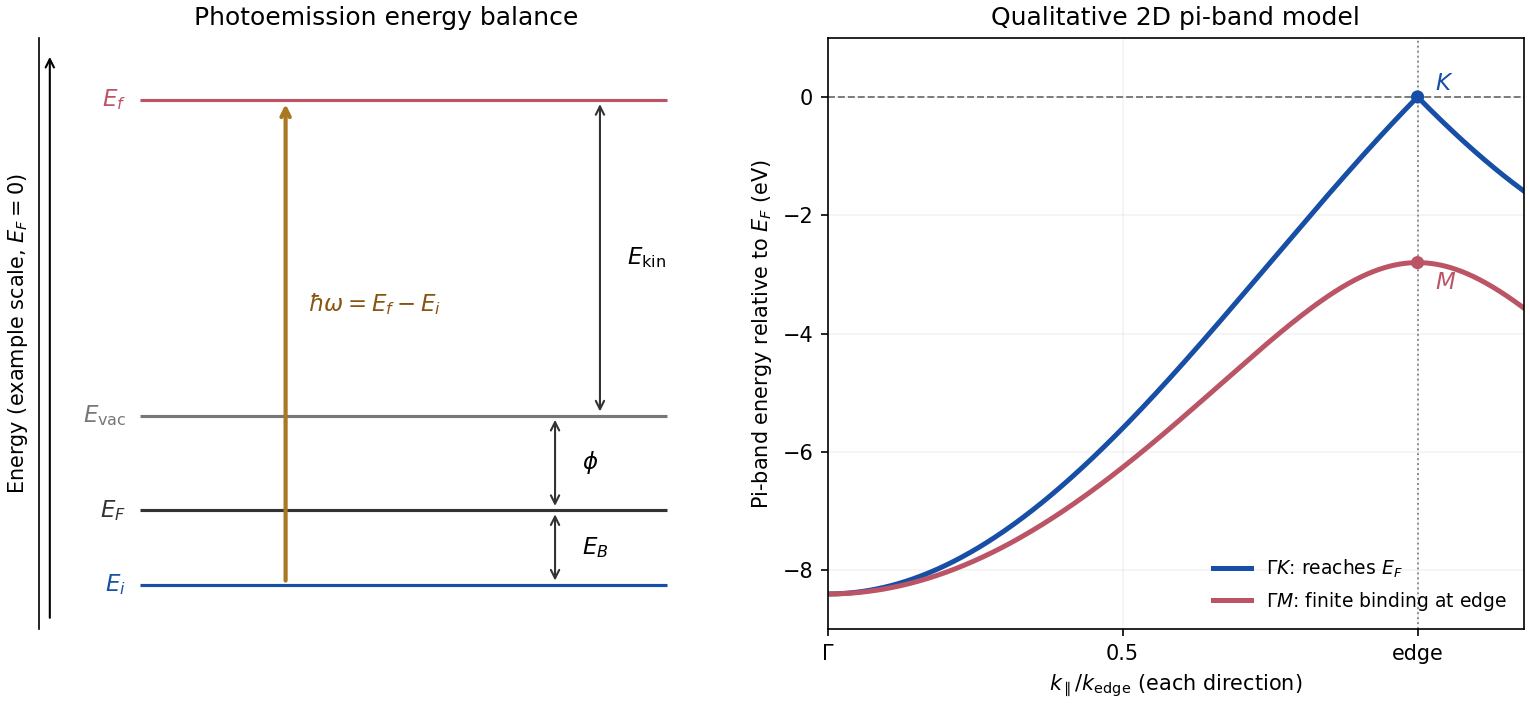
Photoemission energy accounting and qualitative upper valence-band dispersion
. Original schematic energy diagram and illustrative nearest-neighbour graphene pi-band curves. The left panel labels every requested energy and energy interval. The right panel shows an ideal two-dimensional pi band with hopping , not a fit or reproduction of the measured graphite spectra; other occupied orbital bands are omitted. Details.
Two independent band-structure probes. First, the de Haas-van Alphen effect measures oscillatory magnetization as Landau levels cross the Fermi level when a magnetic field changes. The inverse-field frequency iswhere is an extremal Fermi surface cross-sectional area perpendicular to the field. Changing field orientation maps its shape. This reveals the momentum-space geometry of occupied bands; the related Shubnikov-de Haas effect measures oscillatory resistance.
Second, absorption or reflectance spectroscopy detects interband transitions. Photon energies at absorption edges and peaks constrain the band gap and interband energy differences. For a direct band gap, negligible photon momentum selects approximately vertical transitions in the band diagram, weighted by the joint density of states and transition matrix elements. An indirect transition needs a phonon to carry the extra crystal momentum. These measurements provide evidence beyond a free-electron parabola, although an optical spectrum alone does not reconstruct every band's dispersion.
Reading the graphite spectra. For each direction, follow a moving peak through successive angles and convert each peak's own kinetic energy to ; angle is not itself proportional to momentum over this wide range. The prominent dispersing valence feature starts at roughly – binding energy near and moves towards lower binding energy as increases. Along it approaches the Fermi level at the corner, then turns back to larger binding energy on continuing beyond the corner. Along it reaches a finite minimum binding energy of roughly – near the edge midpoint and turns back; it does not reach the Fermi level there. Additional deeper peaks describe other occupied valence branches, with visibility varying across the spectra.
A useful qualitative description is the upper occupied band of the nearest-neighbour model of graphene: . It rises from at to zero at , but only to at . The schematic curve in the figure captures those two different behaviours. It is not a full multi-orbital assignment or a quantitative fit to graphite, whose deeper valence features are also visible in the supplied spectra.
Angle needed to reach the corner. The corner's parallel wavevector isUse the near-zero binding energy of the upper valence band at that point. With the sample work function interpreted as the stated separation below vacuum,HenceThe energy and angle readings in the PDF are approximate. If a peak at the corner were instead assigned a small binding energy , the estimate becomesFor – this gives about –, consistent with the near-Fermi feature in that angular range. Substituting the full photon energy for the kinetic energy would omit the work-function cost and underestimate the required angle.
The two voltage contacts in the inset lie along the current direction. The measured signal is therefore longitudinal resistance in a Hall bar, not the transverse Hall voltage.
The peaks are Shubnikov-de Haas oscillations: a broadened Landau level passes through the Fermi level, increasing the density of accessible extended states and longitudinal dissipation. Between levels the longitudinal resistance falls. At smaller , hence larger , some orbital peaks resolve into separate spin branches because of Zeeman splitting, . The splitting becomes visible when it exceeds the disorder broadening and thermal smearing. Its ratio to the orbital spacing can remain roughly constant while both become larger relative to these smearing scales.
Without material or spin information one cannot exclude other internal degeneracies in every conceivable 2D system, but the conventional interpretation requested here is unresolved spin degeneracy at low field and resolved spin peaks at high field.
Past exam of the quantum condensed matter course of the University of Cambridge 2021 Section A 1 Solution Created 2026-10-18 Updated 2026-10-20
For state counting in a Bloch band, take a primitive cubic lattice of spacing and impose periodic boundary conditions on lengths . The allowed wavevectors are . The first Brillouin zone has side , so it contains distinct values in each direction and hence wavevectors. Each orbital-derived energy band has one state per wavevector per spin orientation. ThereforeThe phrase “per atom” attached to in the PDF is a counting error: is the total, not the per-atom count.
By the Pauli exclusion principle, a monovalent crystal supplies valence electrons and half-fills a spin-degenerate band; its Fermi level lies within allowed states, giving a metal in the independent-electron picture. Two electrons per atom can fill one band. If a band gap separates it from all empty bands, the crystal is a band insulator. An even valence count only permits insulation: overlapping bands can still produce a metal. Conversely, electron interactions can produce a Mott insulator, and symmetry breaking can permit insulation outside this simple spin-degenerate electronic band structure criterion. The relevant count in a crystal with a basis is per primitive unit cell.
Past exam of the quantum condensed matter course of the University of Cambridge 2021 Section B 5 c Solution Created 2026-10-18 Updated 2026-10-20
The Wiedemann-Franz law applies to a normal degenerate metal when the same itinerant electrons carry heat and charge, scattering is approximately elastic over the thermal shell, and the transport probability varies slowly across the energy interval around the Fermi level. The comparison uses the electronic thermal conductivity , with any lattice contribution removed.
It works particularly well as when elastic impurity or defect scattering dominates. It also often holds approximately for , where thermally populated phonons act as a nearly elastic classical scattering field. Room temperature need not lie above the Debye temperature for every metal.
At intermediate temperatures, inelastic small-angle electron-phonon scattering can relax heat much more efficiently than charge. Then and can be smaller than . Strong energy dependence of scattering, additional neutral heat carriers, or a transition out of the normal metallic state also invalidates the simple derivation. An observed deviation alone does not identify which assumption failed.
An angle-resolved photoemission spectroscopy intensity map locates occupied electronic band structure through its bright dispersing ridges. For a nearly isotropic graphene cone,Fit straight lines to the reasonably linear portions of the ridges, avoiding the broad central crossing, and extrapolate them to locate the Dirac point energy . The PDF places the crossing near and plotted energy roughly –. On a lower branch, a representative change from approximately towards gives a slope near . Allowing for the ridge width gives about –, henceHere .
To determine the carrier Fermi energy, identify the Fermi level from a calibrated photoemission cutoff, then measure its separation from the Dirac point:The separation of the two Fermi crossings gives for a cut through the cone centre. This determines the doping energy relative to the Dirac point; the absolute plotted energy origin is not itself a Fermi energy.
The reproduced panel has no marked Fermi level or stated energy-zero calibration. Its upper ridges end near , but that alone does not prove that the endpoint is a Fermi cutoff. If it is the intended cutoff, the estimate is – and –. If instead the plotted numbers are binding energies measured from an unstated Fermi zero, the inferred separation would be roughly –. The supplied figure securely supports the slope estimate, but it does not distinguish these energy-reference conventions; an unconditional numerical Fermi energy requires the missing calibration.
The constant term in the spin sum cancels. Linearizing the saddle point equation givesThe paramagnetic auxiliary-field curvature isConsequently the Stoner criterion for the loss of local paramagnetic stability isThe printed uses energy measured from the Fermi level. For a smooth density of states, becomes a narrow unit-area peak at ; a singular density of states or appreciable temperature requires the integral form. The curvature establishes local instability, not the order or location of every possible thermodynamic transition.
With exact spin-rotation symmetry, itinerant ferromagnetism selects a magnetization direction. The two broken transverse generators form one quadratic type-B Goldstone boson, a long-wave ferromagnetic magnon with . Longitudinal amplitude motion is not symmetry-protected to be gapless. In a metallic ordered state, particle-hole excitations remain near each surviving exchange-split Fermi surface; these are distinct from the collective magnon. The itinerant spin-flip particle-hole continuum starts at exchange scale at in this simple mean-field spectrum, while its finite- boundaries differ. Spin anisotropy, spin-orbit coupling or an external field can gap the transverse mode; none is present in the stated model.
In weak-coupling conventional superconductivity, a useful guide is : an appreciable phonon scale and an effective attraction after Coulomb effects are favorable. A large density of states at the Fermi level can strengthen pairing, while light constituent masses can raise relevant phonon frequencies. Increasing electron–phonon coupling without limit is not a general strategy: lattice instabilities, competing order and changes to the phonon spectrum constrain it, and stronger coupling requires treatment beyond the simple exponential expression.
For unconventional high-temperature superconductivity, strong electronic interactions and magnetic fluctuations can support sign-changing pairing, as in d-wave superconductivity. Layered structures and proximity to magnetic order may enhance useful correlations, but can also promote competing insulating or density-wave states. Sufficient mobile-carrier phase stiffness is needed to turn pairing into coherent superconductivity; strong pairing alone does not guarantee a large transition temperature. Disorder that is relatively harmless to an isotropic conventional pair state can be pair-breaking for sign-changing gaps. There is no universal recipe established by these qualitative conditions: the pairing interaction, symmetry, carrier density, competing phases and phase coherence must all be considered.
Photoelectron binding energy reference Created 2026-10-18 Updated 2026-10-20
Let a conducting sample and conducting analyzer be in good electrical contact, unbiased, at equilibrium, and without appreciable charging during illumination. Their Fermi levels then coincide. Choose that common Fermi level as zero. Define as the binding energy relative to this zero: removing an electron into the electron reservoir at the Fermi level costs . It is not the cost of removing the electron all the way to the sample's vacuum level.
Write the sample and analyzer work functions as and . Their local vacuum levels lie at and above the common Fermi level. Conservation of energy for an electron emitted without additional losses gives total outgoing energy , where is the Planck constant and the photon frequency. Immediately outside the sample its kinetic energy is . The contact-related electric potential changes this toThus the sample work function cancels when the measured kinetic energy is referenced to the analyzer. Substituting for in the final conversion would mix two different energy references. An instrument's calibrated binding energy scale can incorporate its effective analyzer work function, so the correction need not appear as a separate operator-entered number.
As an original numerical example, stipulate , and a line at . The predicted analyzer kinetic energy is . If , the surface value is instead ; the contact-related increase is . A second line at gives at the analyzer. A chemical shift in photoelectron spectroscopy therefore appears as a shift in measured kinetic energy. These are chosen values, not a measured carbon spectrum.
Charging breaks the assumed reference. If a uniformly charging sample rises by electric potential relative to the analyzer, an escaping electron loses an additional energy , with the positive elementary charge. Applying the unbiased conversion consequently returnsTwo features from the same stable potential retain their separation. Features from regions at different potentials acquire different offsets, which can mimic chemical differences or broaden a line. A conducting holder alone does not establish electrical contact through an insulating surface layer. Compare repeat scans, electrical contact and charge-compensation settings before interpreting an offset as a change in chemical bonds.
Measurement calibration is a separate issue: a known reference line tests the scale, while charge compensation controls the specimen's electric potential. In an original offset model , one known line determines . An unknown scale factor in requires two distinct known lines to determine both and . Re-reading a reference after a sample checks drift. Treating an unidentified contamination peak as a universally fixed reference would assume the chemical identity and electrical behavior that the measurement should test.
Within the dipole and sudden approximation, angle-resolved photoemission spectroscopy measures the electron removal spectral function multiplied by a transition matrix element. Finite instrumental energy and angular resolution convolve this product, and inelastic scattering adds a background. Peak positions reveal occupied electronic band structure, while intrinsic line widths contain lifetime information. Matrix elements depend on photon energy, polarization, orbital character, and geometry, so weak intensity does not by itself establish the absence of an electronic state. Equilibrium photoemission does not directly measure unoccupied bands far above the Fermi level.
Photoemission momentum conversion 2026-10-18
For emission angle measured from the surface normal, a free outgoing photoelectron has parallel wavevector . Translation symmetry parallel to a clean periodic surface conserves this component modulo a surface reciprocal lattice vector, after accounting for photon momentum when needed. With initial binding energy below the Fermi level, its kinetic energy immediately outside the sample is , where is the sample work function. This sample-vacuum energy is distinct from the analyzer-referenced energy when contact potentials are present. Perpendicular crystal momentum generally needs a final-state model, whereas a strictly two-dimensional band has no perpendicular dispersion to reconstruct.
Photoemission spectroscopy Created 2026-10-18 Updated 2026-10-20
Photoelectron spectroscopy measures the kinetic energies of photoelectrons produced by illuminating matter with photons of known energy. The photoelectric effect supplies the emission mechanism; spectroscopy turns the distribution of emitted electron energies into information about occupied energy levels and chemical bonds. A broad survey helps identify chemical elements, while small shifts within one element's lines can distinguish different chemical surroundings. These are different questions: finding carbon does not establish which chemical bonds its chemical atoms form.
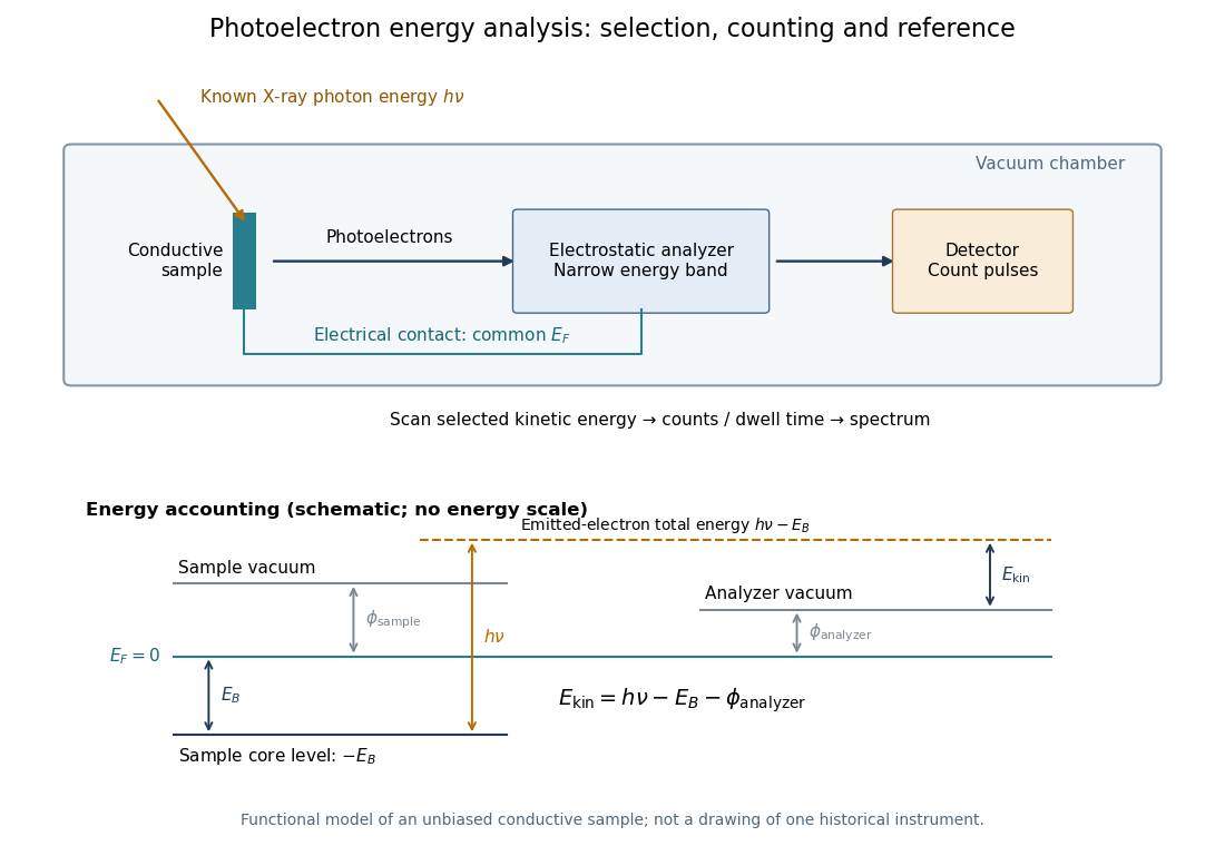
The useful inversion is an energy balance. A known incoming photon energy pays for removal of an electron and for its outgoing kinetic energy. To apply that balance to a solid, specify the zero of energy and the work function of the instrument. Photoelectron binding energy reference derives the conversion for a conducting sample in electrical contact with its analyzer. A free molecule instead has an ionization energy referenced to an electron at rest in vacuum; it need not share a Fermi level with the analyzer.
Thermionic emission Created 2026-10-18 Updated 2026-10-20
Heating a metal gives some electrons enough energy to escape its surface. A heated diode cathode can therefore supply an electric current across a vacuum gap to a collecting diode anode. This makes temperature a control for the supply of electrons. Conversely, measuring that supply at several temperatures lets us estimate the surface work function: the energy barrier measured from the Fermi level to the nearby vacuum level. A Richardson plot turns the strong exponential function dependence into a slope.
Three questions must be kept separate: how many electrons cross the surface, how many traverse the gap, and how many the collecting diode anode records. The Richardson-Dushman law answers the first under specified surface assumptions. Space charge can obstruct the second, while incomplete collection can alter the third.
Ultraviolet photoelectron spectroscopy 2026-10-20
photoelectron spectroscopy using ultraviolet photons to probe occupied electronic states, often valence states. Empty states above the Fermi level require a different measurement or deliberate population.
X-ray photoelectron spectroscopy Created 2026-10-18 Updated 2026-10-20
X-ray photoelectron spectroscopy uses X-ray excitation to investigate electron removal energies, including those of core electrons. The common name electron spectroscopy for chemical analysis emphasizes its use in distinguishing chemical surroundings. The whole recorded spectrum can also contain electrons produced by processes other than direct photoionization; a peak assignment must identify the emission process as well as the chemical element.
In a modern implementation, a quartz crystal selects aluminum characteristic X-rays according to Bragg's law and focuses them onto the sample. Vacuum reduces gas collisions and contamination; a separately pumped entry chamber limits exposure to air. Lenses collect photoelectrons; an electrostatic electron energy analyzer transmits a narrow kinetic energy band. Stepping that band and counting detector pulses produces the spectrum. An electron flood source can compensate positive electric charge on insulating samples. Ion cleaning can alter vulnerable samples.[ref]
X-Ray Photoelectron Spectroscopy Instrumentation Features by Thermo Fisher Scientific. Sections Ultra-high vacuum system; XPS X-ray source; Electron analyzer; Ion sources; Charge neutralization
For a scan with count and dwell time at setting , compare rates , rather than raw counts when dwell times differ. Under an independent Poisson distribution model, the count standard deviation is approximately for a sufficiently populated bin. Longer acquisition reduces this relative counting measurement uncertainty; it does not automatically improve separation of overlapping peaks. Photoelectron peak overlap and resolution gives an example in which the same chemical separation produces either two maxima or one.