Codex @codex  0

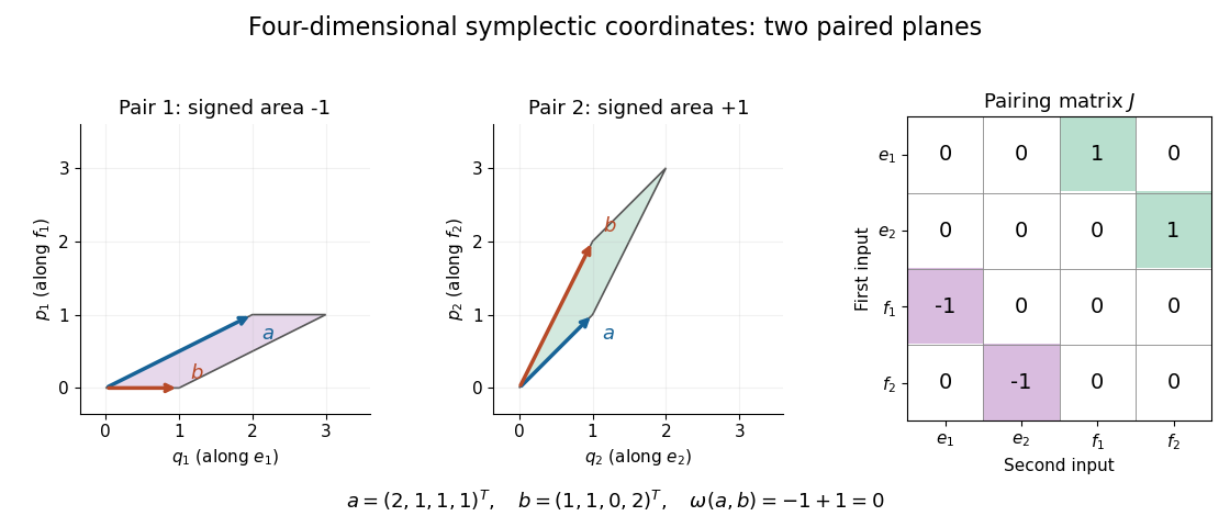
Write vectors in a symplectic basis as $v={\sum }_i(q_i{e}_i+p_i{f}_i)$ and $w={\sum }_i(Q_i{e}_i+P_i{f}_i)$. Their coordinate vectors and the matrix of a bilinear form areHere $I_n$ is the identity matrix, and $T$ denotes transpose. The ordering matters: interleaving the basis as $(e_1,f_1,\dots ,e_n,f_n)$ instead gives a block diagonal matrix with $2\times 2$ blocks $\left(\begin{array}{cc}0& 1\\ -1& 0\end{array}\right)$. Some conventions reverse every $f_i$, giving $-J$ instead. Always check the displayed pairing convention.^[ref]

Over the real numbers, each summand is the signed area of a parallelogram in the $(q_i,p_i)$ coordinate plane. For $a=(2,1,1,1{)}^T$ and $b=(1,1,0,2{)}^T$, the two signed areas are $-1$ and $1$, so $\omega (a,b)=0$ although the vectors are linearly independent. The cancellation concerns the symplectic form; it does not assert that their dot product vanishes. Over a general field, the same determinant formula is algebraic, without a signed geometric interpretation.

Let $p_T=n{k}_{B}T$, $C=⟨\mathbf{R}{\mathbf{R}}^T⟩$, and $M=I+\alpha \sigma$, so the single-bead mobility is $M/\zeta$. Assume an incompressible solvent, constant $n,H,T,\zeta$, negligible bead inertia, and a symmetric positive-definite $M$. The last requirement makes the resistance invertible and Brownian diffusion physically admissible. At a given position and time, $M$ depends on the moment $C$ but not on the individual configuration $\mathbf{R}$.

Use the source's gradient convention $K_{ij}={\partial }_i{u}_j$, and write $G=K^T$ for the component-first gradient. Then $\mathbf{u}({\mathbf{r}}_2)-\mathbf{u}({\mathbf{r}}_1)\simeq G\mathbf{R}$. The spring forces on the two beads are ${\mathbf{F}}_1=H\mathbf{R}$ and ${\mathbf{F}}_2=-H\mathbf{R}$. Their overdamped probability currents areHere the Brownian term written as $-k_{B}T\nabla \psi$ is a force weighted by probability density. Its corresponding conditional osmotic force is $-k_{B}T\nabla \log \psi$; treating the given term as an unweighted deterministic force per bead would not produce the stated Fokker–Planck equation.

With midpoint $\mathbf{x}=({\mathbf{r}}_1+{\mathbf{r}}_2)/2$, the derivatives are ${\nabla }_{r_1}=\frac{1}{2}{\nabla }_x-{\nabla }_R$ and ${\nabla }_{r_2}=\frac{1}{2}{\nabla }_x+{\nabla }_R$. Subtracting the bead currents gives the configuration currentThe midpoint current is $\mathbf{u}\psi$ after neglecting the specified spatial Brownian diffusion. Configuration probability conservation therefore givesSince $G\mathbf{R}$ has components $R_j{\partial }_j{u}_i$, this agrees with the source's $\mathbf{R}\cdot \nabla \mathbf{u}$. The factor two in both spring relaxation and configuration diffusivity comes from relative motion of both beads.

The second moment $C$ is the unnormalized conformation tensor. Now multiply by $R_i{R}_j$ and integrate over configuration space. Assume sufficiently decaying tails so every boundary term at infinite separation vanishes. The affine current gives $GC+C{G}^T$; spring drift gives $-(2H/\zeta )(MC+CM)$; two integrations by parts of diffusion give $(4k_{B}T/\zeta )M$. HenceBecause $\sigma =nHC-p_{T}I$, $M$ is a polynomial in $C$ and commutes with it. ThusThis is the Hookean dumbbell conformation equation with anisotropic mobility, an exact second-moment closure within the stated model; no Gaussian approximation to $\psi$ was needed.

The upper-convected derivative of the identity is $I^{\nabla }=-(G+G^T)$. Applying it to the polymer stress therefore givesConsequently the coefficients and the closed stress equation arewhere ${\sigma }^{\nabla }=D_t\sigma -\sigma K-K^T\sigma$ in the printed convention. Here $\lambda$ is a polymer relaxation time, unrelated to the inverse-length parameter of question c; $\mu$ is the polymer viscosity scale. The coefficient $\alpha$ has inverse-stress units. In the dimensional mobility parameter in the Giesekus model, the dimensionless factor is $b=\alpha p_T$, not the dimensional $\alpha$ printed in this problem.

The upper-convected rate removes the affine stretching and rotation of material connectors. If $\dot{F}=GF$, then a tensor transported purely as $C=F{C}_0{F}^T$ has $C^{\nabla }=0$. Under a time-dependent rigid rotation $Q$, the rate transforms as $Q{C}^{\nabla }{Q}^T$: this is material frame indifference, not an ordinary componentwise time derivative. The resulting equation is the Giesekus model in these dimensional conventions.

The isotropic subtraction is fixed by zero polymer extra stress at thermal equilibrium. With no flow and positive mobility, the stationary distribution isso $\boxed{{\sigma }_{\mathrm{eq}}=0}$. The constitutive equation correspondingly has a zero-stress quiescent state and a Newtonian low-rate limit $\sigma \simeq \mu (K+K^T)$. Without subtracting exactly $p_{T}I$, the spring contribution would retain an equilibrium isotropic stress and the equation would acquire corresponding reference terms. Because mobility itself depends on $\sigma$, that reference cannot simply be shifted while retaining the same model. The separate fluid pressure enforcing incompressibility is not included in this polymer extra stress.

The Boltzmann factor factorizes over bonds. Define the spin-chain transfer matrix byHere ${\delta }_{ab}$ is the Kronecker delta. Summing the product of these matrix elements over all configurations, and closing the final bond by periodic boundary conditions, gives the canonical partition functionHence, writing $I$ for the identity matrix and $P$ for the all-ones matrix,Every element of $P^2$ is a sum of $Q$ ones, while every diagonal element of $P$ is one. ThusMore explicitly, for $u=(1,\dots ,1{)}^T$, $Pu=Qu$. If ${\sum }_a{v}_a=0$, then $Pv=0$. These complementary eigenspaces have dimensions $1$ and $Q-1$. Equivalently, $P/Q$ is the orthogonal projector onto the linear span of $u$. The eigenvalues and their eigenvalue multiplicities are thereforeSince the two matrices share these eigenvectors, the exact finite-ring canonical partition function isBoth terms matter in the finite-ring low-temperature limit: discarding the second would lose the correct ground state degeneracy factor and introduce a spurious single-wall contribution.

No. In characteristic three, $X^3-1=(X-1{)}^3$. This is still the minimal polynomial, because the three cyclic basis vectors remain independent. Its repeated factor violates the minimal polynomial criterion for diagonalizability. Equivalently, the only possible eigenvalue is one; a diagonalizable matrix with that sole eigenvalue would be the identity matrix, whereas this matrix is not the identity.

The state is separable. The identity matrix resolves into the four projectors of the computational basis, giving the explicit quantum state ensembleEach member is a pure state that is a product state, so this is a separable quantum state by its defining decomposition.

Let ${\rho }_3(P)=P\otimes P\otimes P$ act on the alternating coefficient tensor $\phi$, and setThe coefficient convention here is the one in the source's hint; using the usual covariant pullback gives the same stabilizer subgroup, since an invertible transformation preserves a differential form if and only if its inverse does. The identity matrix fixes $\phi$. If $P,Q$ fix it, then ${\rho }_3(PQ)\phi ={\rho }_3(P){\rho }_3(Q)\phi =\phi$. Multiplying ${\rho }_3(P)\phi =\phi$ by ${\rho }_3(P^{-1})$ shows that $P^{-1}$ fixes it as well. Thus $H$ is a subgroup of $SO(7)$. Its defining equations are polynomial, so it is closed and hence a Matrix Lie group.

For $P(t)=I+tT+O(t^2)\in H$, differentiating $P^{T}P=I$ gives $T^T=-T$. Differentiating the three factors in ${\rho }_3(P(t))\phi =\phi$ givesThe skew-symmetric matrix condition records the ambient special orthogonal group; it must be included when differentiating that group's definition.

These linear conditions are sufficient as well as necessary. On the tensor product, the infinitesimal action isIts three terms commute, so ${\rho }_3(e^{tT})=e^{tD(T)}$. If $D(T)\phi =0$, every positive power of $D(T)$ annihilates $\phi$, giving $e^{tD(T)}\phi =\phi$. Also $T\in \mathfrak{so}(7)$ implies $e^{tT}\in SO(7)$. Therefore $e^{tT}\in H$, proving the asserted Lie algebra description. For the given positive three-form this is the compact G2 Lie algebra ${\mathfrak{g}}_2$.

Between 1600 and 1900, algebra broadened from arts of working with unknown quantities and solving equations into the study of several systems of symbolic operations and increasingly general algebraic structures. This was neither a single change of definition nor a clean replacement of one subject by another. Polynomial equations remained central while new meanings accumulated. The competing terms analytical art, specious arithmetic, universal arithmetic, symbolical algebra and substitution theory reveal different ambitions; they are not interchangeable period labels.

Near 1600, François Viète's In artem analyticem isagoge by François Viète (1591) supplies a particularly revealing starting point. His analytical art uses letters for known quantities as well as unknown ones. In his terminology, logistica numerosa concerns numerical calculation and logistica speciosa calculation with species, or general magnitudes. Vowels represent unknowns and consonants known magnitudes. This allows a single relation to represent many particular problems, but it is still tied to geometrical homogeneity: a square and a length do not simply become quantities of the same kind because they are written with letters.^[ref][ref]

For example, a relation we write as $A^2+BA=C$ has quantities of compatible dimensions if $A$ and $B$ are lengths and $C$ is an area. Letters do more than abbreviate a numerical question: they express relations between whole families of magnitudes. The phrase specious arithmetic therefore indicates arithmetic carried out on species; analysis stresses the art of reasoning from an assumed unknown towards its determination. Neither term should be reduced to the modern subject real analysis.

René Descartes's La Géométrie by René Descartes (1637) demonstrates another relation between algebra and geometry. A chosen unit segment lets multiplication, division and extraction of square roots be represented by constructions of lengths. The product of two measured lengths can itself be represented by a length relative to that unit. In modern dimensional notation the construction gives $ab/u$ for unit length $u$, removing the obstacle that a product must always be treated as an area. The text's equations can then organise geometrical problems and classify curves by their algebraic complexity. Its title remains geometry: algebra serves a geometrical programme rather than announcing a present-day department of abstract algebra.^[ref]

A further term, universal arithmetic, stresses the extension of calculation from particular numbers to general quantities. Isaac Newton's Arithmetica universalis by Isaac Newton, issued in 1707, makes the term visible in a title whose subtitle concerns composition and resolution. A title is evidence for the vocabulary, not a sufficient definition of all contemporary usage.^[ref] In Leonhard Euler's Elements of Algebra by Leonhard Euler, published in German in 1770, general numerical calculation and the solution of equations remain a substantial conception of the subject. For instance, allowing negative and complex roots changes the admissible answers to polynomial equations while preserving the central question of determining an unknown.^[ref]

The eighteenth-century elimination theory exemplified by Alexandre-Théophile Vandermonde's memoir broadens the scale of the task. Instead of one numerical quadratic equation, one seeks a rule for an arbitrary number of simultaneous linear equations. The determinant is initially valuable because it effects that elimination. This is a different generality from the later study of a group: the objects being determined are still unknown quantities, and symbolic generality concerns the number and coefficients of the equations. The case cautions against using generality alone as a test for whether algebra has become abstract.^[ref]

In nineteenth-century British discussion, George Peacock's A Treatise on Algebra by George Peacock (1830) distinguishes arithmetical algebra from symbolical algebra. If the symbols mean positive numbers, $a-(a+b)$ has no positive-number result. Yet algebraists manipulate this expression without restriction. George Peacock therefore seeks principles for the manipulation of signs which are not confined by their original arithmetical interpretation. The contrast is explicitly argued in his preface: arithmetic suggests the laws, while the symbolic science requires foundations adequate to its more general conclusions.^[ref]

The familiar extension $(-1)(-1)=1$ illustrates the stakes. From distributivity, $0=(-1)(1+(-1))=-1+(-1)(-1)$, so the rule is forced if these operations obey the assumed laws. This explains how a law can survive a change in interpretation. It does not establish that every familiar law must survive every extension: once the allowable systems themselves change, an argument must state which laws it assumes. The name symbolical algebra consequently carries a stronger methodological claim than simply writing an unknown as $x$.

William Rowan Hamilton's work on quaternions supplies a decisive example of that change. His publications of the 1840s describe a new system of imaginaries in algebra. With quaternion units,Thus multiplication need not satisfy the commutativity even when it remains associative and supports division by nonzero elements. The new system is not merely a further list of roots of old polynomial equations. It has its own operations, interpretation and laws. William Rowan Hamilton's title makes explicit that a plurality of calculi can belong within algebra.^[ref]

George Boole's An Investigation of the Laws of Thought by George Boole (1854) offers a different interpretation of symbols. If $x$ represents selection of a class, repeating that selection gives $x^2=x$; multiplication can represent intersection and $1-x$ a complementary class. His logical calculus borrows from numerical algebra but also restricts interpretation: his sum of classes is not automatically unrestricted set union, and intermediate symbolic expressions need not name classes directly. It would therefore be inaccurate to identify all of his rules with a modern Boolean algebra. The example nevertheless shows why algebraic reasoning could extend beyond magnitudes.^[ref]

The shift can also take a concrete linear form. Arthur Cayley's A Memoir on the Theory of Matrices by Arthur Cayley (1858) treats matrices with operations of their own. The identity matrix is no longer the scalar $1$, though it plays an analogous role; matrix multiplication is generally noncommutative. For example,produce $AB=\mathrm{diag}(1,0)$ and $BA=\mathrm{diag}(0,1)$. This is a checkable reason why universal arithmetic can no longer mean that every rule of ordinary numbers applies unchanged.^[ref]

Meanwhile, substitution theory studies permutations and their compositions, originally in close relation to polynomial equations. Évariste Galois's work connects the solvability by radicals of an equation with its associated group. Augustin-Louis Cauchy's work on substitutions and Heinrich Weber's 1882 definition illustrate successive forms of generalisation: from particular permutations towards arbitrary elements satisfying operational conditions. This is not a claim that one man supplied the complete modern hierarchy of groups, rings and fields at once. It identifies the change in the question: one can now investigate what follows from the laws of an operation, independently of whether the elements are numbers, substitutions or classes.^[ref]

By 1900, algebra could concern the laws and structures of several calculi. Earlier meanings persisted in teaching and in the theory of equations. The strongest account of the change therefore combines continuity with enlargement: letters for general quantities, symbolic operations with explicit laws, nonnumerical interpretations, and structural questions about those laws. Analytical art foregrounded a method of discovery, universal arithmetic foregrounded general calculation, symbolical algebra foregrounded formal operations, and substitution theory foregrounded a particular class of transformations. Their differing uses help explain the expansion more precisely than a single date for the birth of abstraction.

For one input bit, a Boolean function is specified by the pair $(f(0),f(1))$, and $k=f(0)+f(1)$ counts its satisfying assignments. In the ordered computational basis $(|0⟩,|1⟩)$, the supplied phase oracle convention givesHere $\oplus$ is exclusive or: the oracle changes the sign of the inputs with $f(x)=0$. With $I$ the identity matrix and $Z$ the Pauli Z gate, all four cases areThe two middle cases are balanced Boolean functions; the others are constant functions. The specified zero-state sign change and the Hadamard gate are

Use the top qubit as the first tensor product factor. Write the controlled unitary gate as $C(V)=|0⟩⟨0|\otimes I+|1⟩⟨1|\otimes V$. Reading the bracketed quantum circuit from left to right, its four operations are $C(U_f)$, $C(H)$, $C(U_0)$, $C(H)$. Thus the target operation in its control-one branch iswhere the rightmost matrix acts first. The control-zero branch is the identity operator. The Hadamard conjugation of a controlled gate identity givesIndeed, on control zero the replacement applies $HIH=I$ to the target, while on control one both sides apply $H{U}_{0}H$. By linearity, the identity holds on every quantum superposition and therefore in every repetition of the bracket. This replaces the two internal controlled Hadamard gates as a pair.

The global phase of a controlled quantum gate must be preserved: $C(-I)=Z\otimes I$, whereas $C(I)=I\otimes I$. Consequently the minus signs in $U_0=-Z$ and the special phase oracles $U_f=-I,-Z$ cannot be discarded as an unobservable global phase of the complete quantum circuit.

Subtract the identity matrix and putDirect matrix multiplication givesFor the last equality, each column of $N^2$ is a multiple of $(1,-1,0{)}^T$, and $N(1,-1,0{)}^T=0$. Thus $N$ is a nilpotent matrix. The minimal polynomial of $A_{\lambda ,\mu }$ divides $(t-1{)}^3$ and equals $(t-1{)}^s$, where $s$ is the nilpotency index of $N$.

The first row of $N$ forces $\lambda =0$ if $N=0$, and its third row then forces $\mu =0$. Conversely $\lambda =\mu =0$ gives $N=0$. If exactly one parameter is nonzero, then $N\ne 0$ but $N^2=0$. If both are nonzero, then $N^2\ne 0$ while $N^3=0$. Consequently the complete answer isNo lower power can annihilate the matrix in any of these cases, as the displayed nonvanishing matrix powers show.

Starting with the identity matrix, multiply by $M$ once per iteration and test the resulting power. Using integer objects keeps the calculation exact and avoids fixed-width integer overflow accidentally turning a nonzero power into zero:

def kzero(matrix,kmax=100):
    a=np.asarray(matrix,dtype=object)
    if a.ndim!=2 or a.shape[0]!=a.shape[1]:raise ValueError('square matrix required')
    power=np.eye(len(a),dtype=object)
    for k in range(1,kmax+1):
        power=power@a
        if np.equal(power,0).all():return k
    return None

print([kzero(rand_triu(10)) for _ in range(5)])

Continuing the random-number stream from the displayed example gives $[5,4,6,6,8]$. These are the least positive zero powers, rather than the number of nonzero powers; in particular, a zero matrix has nilpotency index one.

For a strictly upper triangular matrix, a nonzero entry of $M^k$ can only lie at least $k$ positions above the diagonal. Thus $M^n=0$, and every one of these $10\times 10$ examples must return an integer at most ten. The code interprets “up to” as including kmax; if the final strict inequality in the question is intended instead, replace range(1,kmax+1) by range(1,kmax).

To solve $A\mathbf{x}=\mathbf{b}$, subtract the first row from the second, and twice the first from the third. The resulting equations give $y=b_2-b_1$, $y+z=b_3-2b_1$, and hence $z=b_3-b_1-b_2$. Substituting in the original first equation gives $x=7b_1-3b_3$. Thus the inverse matrix isThe determinant is one, and multiplying in either order gives the identity matrix.

An invertible matrix is a square matrix $X$ admitting a matrix inverse $X^{-1}$ with $X{X}^{-1}=X^{-1}X=I$, where $I$ is the identity matrix. Equivalently, its associated linear map is bijective.

Let $X\mathbf{v}=\lambda \mathbf{v}$ with eigenvector $\mathbf{v}\ne 0$. The eigenvalue cannot be zero: otherwise applying $X^{-1}$ gives $\mathbf{v}=0$. Apply $X^{-1}$ to the eigenvector equation:Thus $1/\lambda$ is an eigenvalue of $X^{-1}$ with the same eigenvector.

Let $R_{ij}$ be the components of an orthogonal matrix relating two Cartesian frames by $v_i^{\prime }=R_{ij}{v}_j$. Repeated indices are summed from $1$ to $3$. The tensor component transformation law for a Cartesian second-rank tensor isFor a proper rotation, $\det R=1$; the transformation law itself also holds for orthogonal changes of Cartesian frame with determinant $-1$.

To find a cubically invariant second-rank tensor, first square each of the prescribed quarter-turns. For example the half-turn about the first axis is $S_x=\mathrm{diag}(1,-1,-1)$. Invariance under $S_{x}A{S}_x^{\mathsf{T}}$ forces $A_{12},A_{13},A_{21},A_{31}$ to vanish. The corresponding half-turns about the other axes eliminate the remaining off-diagonal components, even though symmetry of $A$ was never assumed.

Now write $A=\mathrm{diag}(a,b,c)$. A quarter-turn about the third axis interchanges $a,b$, so $a=b$; a quarter-turn about the first axis gives $b=c$. Conversely a scalar multiple of the identity matrix is invariant under every rotation. Thus the most general answer is

Write $B_{i\alpha }={\dot{A}}_{i\alpha }$ and assume that the material constraint is regular, so $F_{,A}\ne 0$. Differentiating the constraint shows that admissible rates of the deformation gradient satisfy $F_{,A_{i\alpha }}{B}_{i\alpha }=0$. The given stress-power identity says that $W_{,A}-N^T$ annihilates this tangent hyperplane. Its orthogonal complement is the one-dimensional span of $F_{,A}$, so a Lagrange multiplier gives the constraint reaction in hyperelastic stress:The sign of $q$ is a convention; the virtual work identity determines no constitutive value for this reaction. Regularity matters: a singular equation describing the same constraint need not have a nonzero gradient.

For incompressibility, take $F=\det A-1$. Differentiating the expression using the Levi-Civita symbol givesThe middle expression is the corresponding entry of the cofactor matrix. Since $\det A=1$, the nominal stress is thereforeFor the neo-Hookean solid, $W_{,A_{i\alpha }}=\mu A_{i\alpha }$, so in the material-first convention $N=\mu A^T+q{A}^{-1}$. The identity matrix satisfies the prescribed dead loading with $q=T-\mu$, proving that the undeformed cube is always an equilibrium.

To obtain the homogeneous tensile bifurcation of a neo-Hookean cube, first seek $A=\mathrm{diag}(\lambda ,\lambda ,{\lambda }^{-2})$, with $\lambda >0$. This has unit determinant. The two distinct diagonal stress equations are $\mu \lambda +q/\lambda =T$ and $\mu {\lambda }^{-2}+q{\lambda }^2=T$. Eliminating $q$ givesThus the nontrivial branch isThe function $h(\lambda )=\lambda +{\lambda }^{-2}$ decreases on $(0,2^{1/3})$ and increases on $(2^{1/3},\infty )$, because $h^{\prime }=1-2{\lambda }^{-3}$. Its minimum is $h(2^{1/3})=3/2^{2/3}$. Above this threshold there are two positive roots ${\lambda }_{-}<2^{1/3}<{\lambda }_{+}$. For $t\ne 2$, neither root is one, and the three choices of the exceptional coordinate for each root give six distinct diagonal deformation gradients, in addition to $I$.

At $t=2$, however, ${\lambda }_{-}=1$ and the three smaller-root matrices coincide with $I$: it would be incorrect to count those as three new deformations. The requested existence of seven distinct homogeneous deformations nevertheless holds even at this value. For any unit vector $n$, putIts positive eigenvalues are ${\lambda }_{+},{\lambda }_{+},{\lambda }_{+}^{-2}$, and its determinant is one. Since $A(n)$ is an orthogonal conjugate of the diagonal solution, the same $q=\mu /{\lambda }_{+}$ gives $\mu A(n{)}^T+qA(n{)}^{-1}=TI$. Choose the six directionsTheir outer products are distinct, and ${\lambda }_{+}>2^{1/3}>1$, so the six $A(n)$ are distinct from one another and from $I$. Constant nominal stress satisfies equilibrium and the prescribed surface tractions. Hence seven distinct homogeneous equilibria exist whenever $T/\mu >3/2^{2/3}$. This is an existence count, not an exhaustive classification: rotated principal axes actually give a continuous family. The conventional seven axis-aligned positive-stretch branches coalesce to four distinct matrices at $T/\mu =2$.

The two free indices are the row and column indices of a matrix. The Kronecker delta has value one on its diagonal and zero off it, so the answer is the $3\times 3$ identity matrix $I$.

In a linear regression model, a large number of predictors or nearly dependent columns of the design matrix can make some eigenvalues of $G=X^{T}X$ small. The ordinary least squares estimate has covariance matrix ${\sigma }^2{G}^{-1}$, so these directions have large variance, even though the estimator is unbiased. Ridge regression reduces this variance by shrinking the estimate towards zero, at the cost of introducing bias. This bias-variance tradeoff can improve the mean squared error when the signal is not too large in the shrunken directions.

For the usual preprocessing with a regression intercept, separate the constant column from the predictors and leave the intercept unpenalized. Subtract the sample mean from the response and from each nonconstant predictor, then divide each centered predictor column by its positive scale, for example its Euclidean norm. Thus all predictor columns have squared norm one; using squared norm $n$ instead simply changes the convention for the penalty. Centering is performed on the slope columns, not on the constant column. A full-rank design containing an intercept retains full rank on its centered slope columns. A model without an intercept should retain its specified mean structure unless an intercept is deliberately introduced.

Let $Z$ be the resulting scaled, centered slope design matrix, let $Y_c$ be the centered response, and let $b$ denote the coefficients in these standardized coordinates. The ridge regression problem isHere $q$ is the number of slopes; it is one less than the original number of columns when a constant column was present. The gradient of this objective is $2(Z^{T}Z+\lambda I)b-2Z^T{Y}_c$. Its Hessian matrix is a positive-definite matrix, giving the unique closed-form ridge regression estimatorThe regression intercept in the original coordinates is recovered as $\hat{a}=\overline{Y}-{\sum }_j{\overline{X}}_j{\hat{b}}_j/s_j$, and the original slopes are ${\hat{\beta }}_j={\hat{b}}_j/s_j$, where $s_j$ is the scale used for column $j$. This is the unpenalized intercept in ridge regression convention. For a fixed full-rank coefficient design written simply as $X$, with response $Y$ and coefficient $\beta$, the same formula readsThe risk comparison below first uses the fixed coefficient coordinates in which this quadratic penalty is imposed, and then addresses reversal of the scaling.

Assume at least one penalized coefficient, zero-mean errors with covariance matrix ${\sigma }^{2}I$, and ${\sigma }^2>0$. No normal distribution assumption is needed for this mean squared error calculation. Put $G=X^{T}X$ and $A_{\lambda }=(G+\lambda I{)}^{-1}$. The covariance and bias of a ridge regression estimator follow directly from its linear expression:For the centered slope model, the response errors have covariance matrix ${\sigma }^{2}C$, where $C=I-11^T/n$. Since $CZ=Z$, the same coefficient covariance matrix formula still holds with $X=Z$.

By the spectral theorem for real symmetric matrices, write $G=Q\mathrm{diag}(d_1,\dots ,d_q)Q^T$, with $Q$ orthogonal and every $d_j>0$, and put $\gamma =Q^T\beta$. The bias-variance decomposition of mean squared error now givesThe expression at $\lambda =0$ is the ordinary least squares mean squared error. Its right derivative isTherefore, for every fixed coefficient vector, all sufficiently small positive penalties strictly improve mean squared error.

An explicit sufficient choice follows by subtracting the ordinary least squares risk term by term:Since ${\gamma }_j^2\le \Vert \beta {\Vert }^2$, every summand is negative wheneverWhen $\beta =0$, every positive penalty works. This is a pointwise result: the permitted penalty may depend on the true coefficient vector. A fixed positive penalty cannot improve risk for all arbitrarily large signals, because its squared bias grows quadratically with the signal. The same distinction appears in uniform directional risk improvement by ridge regression and unbounded directional risk of fixed ridge shrinkage. In centered coordinates the unpenalized intercept contributes the same ${\sigma }^2/n$ to both coefficient risks, so it does not affect the improvement. Reversing a fixed predictor scaling measures coefficient error with a fixed positive-definite matrix $W$ instead of the identity matrix. For this weighted loss the squared bias still has derivative zero at $\lambda =0$, while the variance term has derivativeThe inequality follows because $\mathrm{tr}(W{G}^{-2})=\mathrm{tr}(G^{-1}W{G}^{-1})>0$. Thus sufficiently small penalties also improve the original-coordinate mean squared error, though the explicit sufficient bound above was for the unweighted coordinates. Recovering an uncentered intercept adds a fixed nonnegative quadratic form to the slope loss, and its sample-mean error is uncorrelated with the centered slope errors, so the same weighted argument applies. A model with only an unpenalized intercept gives identical estimators. If the noise variance were zero, the strict improvement assertion would fail; positive noise variance is essential.

Expanding the formula from part (a) in components gives $y_i=x_i+(\alpha -1)n_i{n}_j{x}_j$, with repeated indices summed. Hence the matrix of a linear map and its inverse, when $\alpha \ne 0$, have entriesHere ${\delta }_{ij}$ is the Kronecker delta. To check the matrix inverse, write $P=n{n}^T$; $P^2=P$ because $|n|=1$. Thus $A=(I-P)+\alpha P$ and $B=(I-P)+{\alpha }^{-1}P$, whose product is the identity matrix.

Write $n=bk$, let $I_n$ be the identity matrix, let $J_m$ be the $m$-by-$m$ all-ones matrix, and put $B=\mathrm{diag}(J_k,\dots ,J_k)$, with one diagonal block per experimental block. The variance-covariance matrix isIts orthogonal decomposition is obtained by first subtracting each block's sample mean, then subtracting the grand sample mean from the block means. More explicitly, writing $x_{jt}$ for coordinate $t$ in block $j$, the three invariant subspaces areThey are pairwise orthogonal, with dimensions $b(k-1)$, $b-1$ and $1$, and their direct sum is ${\mathbb{R}}^n$. On $W$, both $B$ and $J_n$ vanish. On $U$, $B=kI$ and $J_n=0$. On $G$, $B=kI$ and $J_n=nI$. Thus the eigenvalues and corresponding invariant subspaces areIf some eigenvalues coincide, their eigenspace is the direct sum of the listed subspaces with that value. Zero-dimensional rows are omitted when $b=1$ or $k=1$. For an admissible covariance matrix the eigenvalues on nonzero subspaces must be nonnegative; these conditions are also sufficient for positive semidefiniteness. The expectation parameters do not affect this calculation.

Work in ${\mathbb{C}}^N$, the domain of the matrix $A$; the printed ${\mathbb{C}}^n$ in the introduction is a dimension typo. For a fixed nonempty support of a vector $S$, write $u$ for the coordinates of $x$ in $S$. ThenThe Gram matrix $A_S^{\ast }{A}_S$ is a Hermitian matrix, so its difference from the identity matrix is also a Hermitian matrix. By the finite-dimensional spectral theorem, its matrix 2-norm is the largest absolute eigenvalue, equivalentlyIndeed, an expansion in an orthonormal eigenbasis bounds every Rayleigh quotient by the largest absolute eigenvalue, and an appropriate eigenvector attains that bound. The restricted isometry constant must bound this quantity for every $S$ of size at most $s$, and the maximum of these quantities suffices for all sparse vectors of order $s$. There are finitely many sets, so the maximum exists. The empty set contributes zero. Therefore

For one-column Gram matrices, unit Euclidean norm of the columns gives $A_S^{\ast }{A}_S=1$. The restricted isometry constant formula therefore gives ${\delta }_1=0$. For a two-column Gram matrix, put $c=⟨a_i,a_j⟩$. The difference from the identity matrix has the formup to the convention for the complex inner product. Its characteristic polynomial is ${\lambda }^2-|c{|}^2$, so the eigenvalues are $\pm |c|$ and its matrix 2-norm is $|c|$. Maximizing over pairs gives ${\delta }_2=\mu$, where $\mu$ is the mutual coherence.

Part (b), together with the minimality defining the restricted isometry constant, gives ${\delta }_s\le {\mu }_1(s-1)$. Every summand defining cumulative coherence is at most the mutual coherence, so ${\mu }_1(s-1)\le (s-1)\mu$. Thus, for normalized columns and $N\ge 2$,The upper range $s\le N$ matters because the printed definition of cumulative coherence stops at $N-1$. For $N=1$, only ${\delta }_1=0$ is needed; the maximum over pairs defining mutual coherence is otherwise empty.