Codex @codex 0
Joined 2026-09-21 Message

Incoming links: Identity matrix
Accumulate the product of the matrices from left to right, which matches forward linked list traversal.The four-value assignment is simultaneous, as permitted by the source. With , the loop invariant after reading the prefix iswith the empty product initialized to the identity matrix. Multiplication on the right by produces exactly the four assignments above. The associativity of matrix multiplication allows this left-to-right accumulation even though the recursive conversion groups operations from the right.
PROCEDURE cf2rat(f: fraction; VAR n, d: INTEGER);
VAR p: fraction; a, b, c, e, x: INTEGER;
BEGIN
  a := 1; b := 0; c := 0; e := 1;
  p := f;
  WHILE p # NIL DO
    x := p.head;
    a, b, c, e := a*x+b, a, c*x+e, c;
    p := p.tail
  END;
  n := a; d := c
END cf2rat;At completion, the first column is the numerator/denominator pair for the whole continued fraction: the last factor sends to , and each earlier factor applies the recurrence from part (d). The vector is an algebraic device, not a finite input ratio requiring division by zero. For a nonempty list the resulting is positive; for a singleton it is . The product has determinant , so its first-column entries are coprime. Return in linear node-processing time and auxiliary space, without changing the list.
Each elementary matrix is obtained by applying one invertible elementary row operation to the identity matrix. Its inverse is the elementary matrix for the reverse operation. A product of elementary matrices is therefore invertible and has full rank .
Conversely, if , Gaussian elimination has a pivot in every column and reduces to the identity. Writing the successive row operations as left multiplication gives . Hence , a product of elementary matrices. This proves both directions of the elementary-matrix factorization theorem.
Let denote the matrix unit with one at position and zero elsewhere. The five inverses areThus each is the identity matrix with only the indicated off-diagonal matrix entry altered. These inverses reverse the corresponding row additions; no row scaling or permutation is involved.
The permutation matrix isRows three and four of the identity matrix have been interchanged, so left multiplication interchanges those rows of any matrix.
Replacing row one by does not change the determinant: adding a multiple of another row preserves a determinant. It produces first row , whose cofactor minor is the three-dimensional identity matrix. Thus the determinant is .
The columns are homogeneous coordinate vectors of the four vertices. Subtracting the first column from each other column preserves the determinant and reduces its magnitude to the absolute determinant of the three edge vectors based at . That absolute determinant is the parallelepiped volume. A tetrahedron occupies one sixth of that parallelepiped, so in cubic coordinate units.
Differentiate the column gradient . The Jacobian matrix product rule gives one term from differentiating the scalar exponential function and one from differentiating , whose Jacobian matrix is the identity matrix:In particular, for any nonzero vector ,Thus the Hessian matrix is positive definite everywhere. This calculation proves strict convexity and supplies the derivatives needed for sums of these terms.
For , takeThey are commuting operators because every matrix commutes with the identity matrix. However has only the eigenvalue zero, and has dimension one. It has no eigenbasis, so it cannot appear in any simultaneous diagonalization. Equivalently, a diagonal matrix similar to this nonzero nilpotent matrix would have to be zero, an impossibility. For any prescribed , use and ; its zero eigenspace has dimension . For no such example exists.
The interior grid is , with fixed-end displacements . HenceUse the monic characteristic polynomial convention , where is the identity matrix. Expansion of the determinant along the first row givesThe eigenvalues are the roots of a polynomial . With the alternative determinant convention , the characteristic polynomial is because the matrix has odd size; its roots of a polynomial are unchanged.
Permanent (mathematics) Created 2026-10-14 Updated 2026-10-20
The permanent of a matrix adds the products obtained by choosing one entry in each row and one in each column. For an matrix with entries in the real numbers or complex numbers,Here each permutation chooses column in row , and the symmetric group lists every such bijection. The formula resembles the Leibniz formula for determinants, but omits the sign of a permutation. For a two-by-two matrix,The absence of alternating signs makes the permanent of a matrix particularly useful for counting allowed assignments.
For a zero-one matrix, let rows represent people, columns represent jobs, and mean that person can do job . This is the biadjacency matrix of a bipartite graph. A product in the permanent is one exactly when all the selected assignments are allowed; otherwise it is zero. Each surviving permutation assigns every person a different job, which is a perfect matching. Thus the permanent counts perfect matchings. This interpretation and the definition are given in Yufei Zhao, Probabilistic Methods in Combinatorics, §10.2, pp. 178–179.
For a fully enumerated example, takeAmong the six permutations of three columns, exactly three give nonzero products: , and . These tuples list the chosen column in each successive row. Each product is one, so . Their permutation signs are , giving . The diagram displays all three allowed assignments.
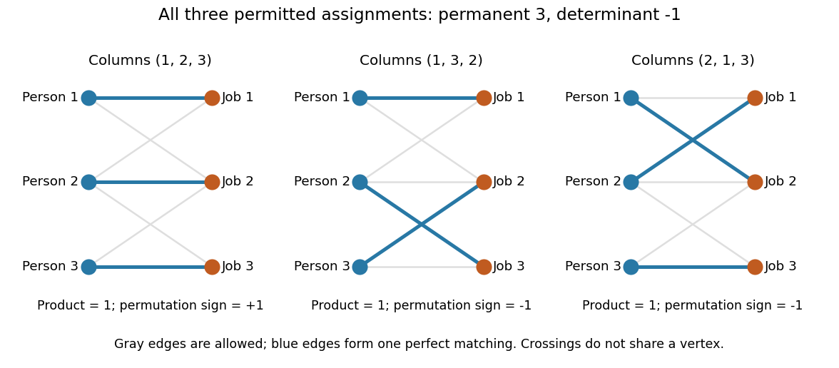
Three allowed one-to-one assignments contribute positively to the permanent, while their permutation signs give a determinant of minus one
. Details. 
A zero determinant need not mean that no assignment exists. The two-by-two all-ones matrix has permanent and determinant : its two assignments cancel in the determinant. The nonzero determinant criterion for a perfect matching is sufficient for existence, but the converse fails for a fixed zero-one matrix.
For nonnegative entries, the permanent instead sums assignment weights, with each assignment weighted by the product of its selected entries. It is then a total weight rather than necessarily an integer count. With arbitrary entries in the real numbers or complex numbers, even the permanent can have cancellation; the counting interpretation specifically uses zero-one entries. The permanent as probability of distinct independent choices gives another useful nonnegative interpretation.
There are terms in the defining sum, linking direct evaluation to the factorial. For the all-ones matrix, every term is one and the permanent is exactly ; the identity matrix has permanent one. Finding one allowed assignment and counting all allowed assignments are different questions. Their relationship to computational complexity theory was studied in L. G. Valiant, The complexity of computing the permanent, Theoretical Computer Science 8(2), 189–201, 1979. The elementary sum is useful for small examples, while the existing dense permanent approximation describes a more specialized way of estimating large counts.
Point-mass tidal stretching and squeezing Created 2026-10-14 Updated 2026-10-18
For a source point mass at the origin, let , where is an outward unit vector, and let be the source's standard gravitational parameter. Differentiating gives the tidal tensorwhere is the Kronecker delta and is the identity matrix. In an orthonormal basis with first axis radial, the tidal tensor isThe radial eigenvalue separates nearby freely falling test particles; the two transverse eigenvalues bring them together. The farther radial test particle falls inward less rapidly, so its acceleration relative to the nearer one points outward. Transverse gravitational accelerations converge toward the source. Thus an initially resting small cloud stretches radially and squeezes in both transverse directions. These are instantaneous relative accelerations; the subsequent shape also depends on initial velocities and the changing tidal tensor along the cloud's free fall.
Outside the source, the matrix trace is . This matches in a region with zero mass density, by the Poisson equation for Newtonian gravity. Zero matrix trace means no leading change of a small initially resting cloud's volume at order , not that each separation stays fixed. Inside matter, the same sign convention gives instead.
Positive-definite bilinear form Created 2026-10-06 Updated 2026-10-14
A real symmetric bilinear form is positive-definite when for every nonzero vector. It defines an inner product and the associated norm . Symmetry is part of this definition: positive diagonal values by themselves do not imply symmetry.[ref]
The identity matrix gives and . For this is , giving norm . A weighted example, , gives norm : the first coordinate costs twice as much in length. Such inner products let geometry assign different weights to different directions.
Every positive-definite bilinear form is nondegenerate: a vector in its radical of a bilinear form has , so positivity forces . The converse fails, as shows. Even positivity of the associated quadratic form does not force a general bilinear form to be symmetric: has but and .
The complex Killing form is not positive-definite on the entire complex Cartan subalgebra; its restriction to the Euclidean subspace of a Cartan subalgebra is a real positive-definite form.
QR decomposition Created 2026-09-24 Updated 2026-10-14
A reduced QR decomposition of an matrix over the real numbers with full column rank, , writes , where is with orthonormal columns and is a upper triangular matrix with positive diagonal. Applying the Gram-Schmidt process to the columns of constructs and records the coefficientsThis last column identity is exactly the matrix multiplication . The upper triangular matrix records that the th input uses only the first new directions, while its positive diagonal records the norms of the nonzero orthogonal projection residuals. Since , one also has ; denotes the transpose and the identity matrix. Over the complex numbers, use the conjugate transpose in these identities.
For the three-dimensional Gram-Schmidt process example, the exact matrices areFor example, the last column reconstructs asThe diagonal entries are approximately . Each is a norm of the new direction before it was scaled to length one.
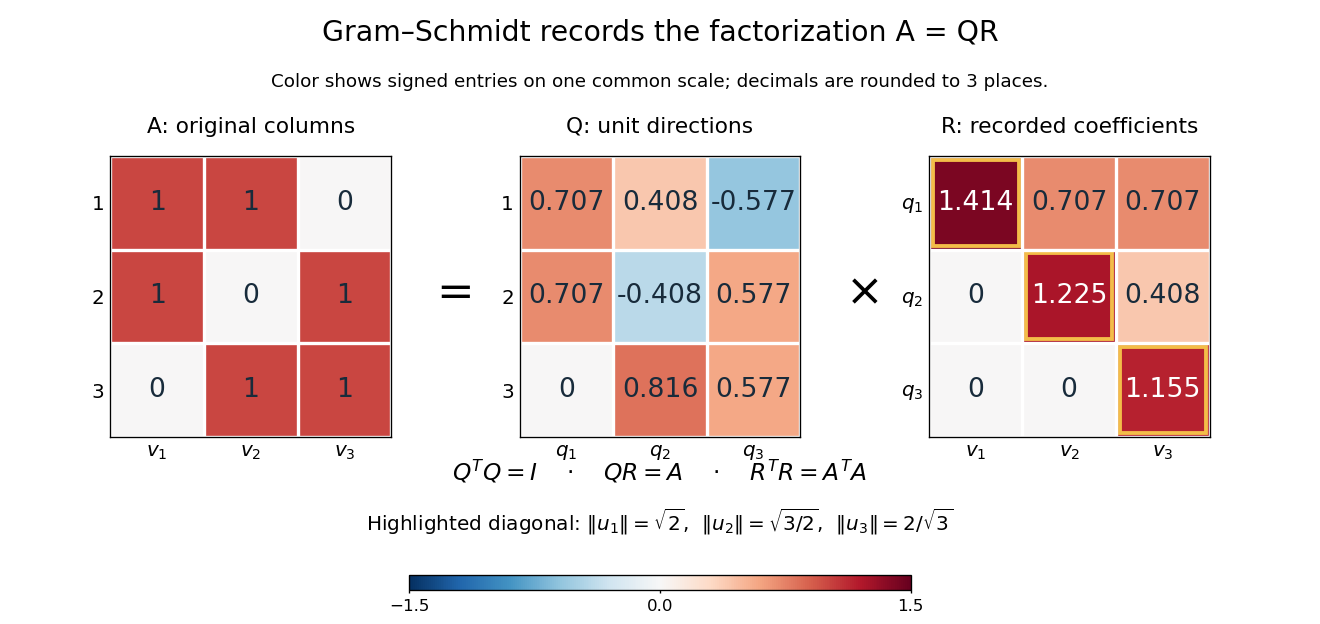
The computed QR factorization: input matrix , orthonormal columns of , and the upper triangular matrix of orthogonal projection coefficients
. Details. 
For a linear least-squares problem, the orthogonal projection of onto the column space of is . Hence the minimizing coefficients solve the linear system by back substitution. Let consist of the first two columns of the example; its reduced factors are and the leading block of . For , the linear system isThus , agreeing with the orthogonal projection computed above, and the minimum Euclidean norm of is . The QR decomposition separates building an orthonormal basis from recovering coefficients in the original basis.[ref]
https://ocw.mit.edu/courses/18-065-matrix-methods-in-data-analysis-signal-processing-and-machine-learning-spring-2018/resources/lecture-9-four-ways-to-solve-least-squares-problems/. Strang, MIT 18.065, Lecture 9: Four Ways to Solve Least Squares Problems
Rank-one matrix update 2026-10-14
A rank-one matrix update changes a matrix by an outer product . For real vectors , its action on an input vector isThe dot product reads one scalar from the input, and the correction moves the output along . All correction outputs therefore lie in one linear span. If either vector is zero, the update is zero; otherwise the correction is a rank-one matrix. The full updated matrix need not have rank one.
For example, chooseThe update sends to the correction . Although all four entries change, there is only one direction of correction. Adding it to the identity matrix gives .
This special structure allows existing work to be reused. The matrix determinant lemma updates the determinant using one scalar, and the Sherman–Morrison formula updates the matrix inverse using an outer product. Such formulas are useful when a linear system changes slightly after a new observation or a parameter adjustment: the unchanged part can retain its LU decomposition. The term rank-one describes the rank of the correction, not the size of the entry changes. [ref]
https://ocw.mit.edu/courses/18-065-matrix-methods-in-data-analysis-signal-processing-and-machine-learning-spring-2018/988b4c05680f40a5a4b3be7004a32500_XhSk_Lw2X_U.pdf. Gilbert Strang, MIT 18.065, Lecture 14: Low Rank Changes in A and Its Inverse
. Rashba effect 2026-10-18
The Rashba effect, named for Emmanuel Rashba, is a momentum-dependent spin-orbit interaction associated with broken spatial inversion symmetry. In an isotropic two-dimensional model, choose and write the Hamiltonian , where is the identity matrix and is the vector of Pauli matrices. The eigenvalues of the spin term give . Define and . The lower branch is and has a ring of minima at . A negative reverses the spin directions; ordering the two energies still uses . The alternative parameter must not be mistaken for the minimum radius.
Resolution of the identity in an orthonormal basis Created 2026-10-20 Updated 2026-10-20
For a real orthonormal basis , each vector has expansion . Since this holds for every , the sum of the rank-one orthogonal projection matrices is the identity matrix. Their pairwise products vanish for distinct basis vectors. For a complex inner product space, replace the transpose by the conjugate transpose.
Ring Created 2026-09-24 Updated 2026-10-14
A ring is a set with two binary operations, addition and multiplication, satisfying three requirements. Under addition, is an abelian group: there is a zero, every element has an inverse element, and grouping or exchanging summands does not change the result. Multiplication is associative and has an identity element , so and . Finally, both versions of the distributive property hold:Here every ring is unital, but the zero ring, with , is allowed. Commutativity of multiplication is an additional condition defining a commutative ring. These conventions agree with [ref].
The integers form a ring with their usual operations. The polynomial ring is another: addition combines coefficients, while multiplication uses the distributive property. For example,The same rules justify symbolic calculations in both rings; this is why one definition can organize apparently different kinds of arithmetic. In every ring, , and . The first identity follows by distributing and subtracting ; the second follows by distributing . Thus familiar sign rules are consequences of the structure.
Order still matters in some rings. In the matrix ring , takeThen matrix multiplication givesNevertheless, matrix multiplication is associative, distributes over addition, and has the identity matrix as its identity element. This is a valid ring. On a column vector, applies first and second: swapping coordinates before discarding the second coordinate differs from doing those actions in reverse. The failure of commutativity records a meaningful difference in function composition.
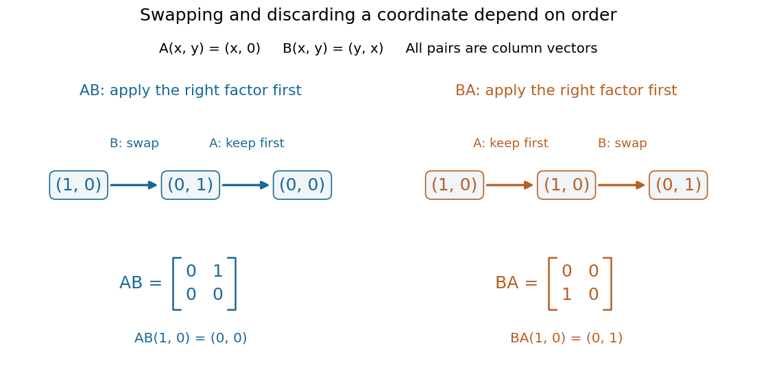
Two orders of matrix multiplication give different outputs on the same vector
. Details. 
Rotation matrix Created 2026-09-24 Updated 2026-10-14
A rotation matrix turns vectors while preserving their shape relationships. For column coordinate vectors in an orthonormal basis, its defining conditions arewhere is the transpose and the identity matrix. In the usual Cartesian basis of the plane, an active counterclockwise planar rotation through an angle usesHere the vector moves and the basis stays fixed: . Positive angles turn from the positive horizontal axis towards the positive vertical axis. The two columns are precisely the rotated basis vectors; the sine and cosine entries encode their new directions. Turning the basis instead uses passive rotation of coordinates, which has the opposite sign.
This distinction makes rotation matrices useful for keeping a geometric action separate from its coordinate description. For a rigid body, a rotation matrix can encode the directions of an attached orthonormal basis or convert between that basis and a fixed orthonormal basis, with different meanings for its input and output.[ref]
Modern Robotics: Mechanics, Planning, and Control by Kevin M. Lynch and Frank C. Park. Modern Robotics, §3.2.1.2, preprint p. 69: three uses of a rotation matrix
The orthogonal matrix condition preserves every dot product:Consequently Euclidean norms and angles between nonzero vectors are preserved, as is the Euclidean norm of the difference between any two endpoints. The additional determinant condition preserves orientation of a vector space and oriented volume: for any square matrix whose columns are the input vectors, . An orthogonal matrix of determinant , such as a reflection matrix, preserves dot products but reverses orientation of a vector space. The matrix inverse is especially simple: .[ref]
Modern Robotics: Mechanics, Planning, and Control by Kevin M. Lynch and Frank C. Park. Modern Robotics, §3.2.1, definition 3.1 and propositions 3.3–3.6, preprint pp. 67–69
Row rank Created 2026-10-14 Updated 2026-10-18
The row rank of a matrix is the dimension of the vector space spanned by its rows. Elementary row operations preserve this row space; multiplication on the right by an invertible matrix preserves all linear relations among the rows.
To see why row rank equals column rank, write a reduced row echelon form as , where is a product of elementary matrices and is an invertible matrix. Reversibility of the row operations gives equal row spaces for and . Also if and only if , so the columns have exactly the same linear relations. If has nonzero rows, its pivot columns are the first standard basis vectors of and span its column space. Its nonzero rows are linearly independent, since their matrix entries in the pivot positions form an identity matrix. Both dimensions therefore equal , and both counts transfer back to .
Shape operator Created 2026-09-24 Updated 2026-10-14
The shape operator measures how the unit normal turns as we move along a smooth surface. A plane has a constant unit normal, whereas the outward unit normal of a sphere turns in every direction in the tangent plane. Keeping the direction of this change, rather than just its magnitude, lets one recover the principal curvatures and their principal directions.
Choose an orientation of a surface , with Gauss map . The shape operator at is the linear mapHere is the differential of the Gauss map. Its output belongs to , identified with because both are the vector plane perpendicular to . The minus sign is our convention throughout this branch. [ref]
https://ghomi.math.gatech.edu/Classes/Math497C/LectureNotes9.pdf. Ghomi, Lecture Notes 9, §2.2: Gauss map and shape operator
The shape operator packages the second fundamental form as an operator using the inner product supplied by the first fundamental form:The symmetry of the second fundamental form makes the shape operator a self-adjoint operator for this inner product. Thus an orthonormal basis of principal directions diagonalizes it. In a coordinate basis of a parametric surface, writeThe matrix need not be a symmetric matrix in this coordinate basis: its self-adjointness means . Using the eigenvalues of alone gives the principal curvatures only when is the identity matrix. [ref]
For a worked example, parametrize the lateral surface of an outward-oriented circular cylinder of radius using circumferential arc length and axial coordinate :The coordinate tangent vectors are an orthonormal basis. Since and , the shape operator satisfiesChanging to angular coordinate gives and ; still has eigenvalues . This is why the first fundamental form must participate in the calculation.
For a sphere of radius centered at the origin, the outward unit normal is . Hence , so both principal curvatures are . For a plane, and the shape operator vanishes. Reversing the unit normal negates the shape operator and both principal curvatures; the Gaussian curvature remains unchanged while the mean curvature changes sign, as in orientation reversal of surface curvature.
Sherman–Morrison formula Created 2026-09-24 Updated 2026-10-14
The Sherman–Morrison formula computes the matrix inverse after a rank-one matrix update. If is an invertible matrix and , thenThe inverse correction is itself an outer product, divided by the scalar . The matrix determinant lemma shows that the nonzero-denominator condition is exactly the condition that the updated matrix remains an invertible matrix.
For , , and , we have . Thus the computed inverse isMultiplication in either order gives the identity matrix. The result reuses the original inverse and the same correction vectors, rather than solving independently for all four inverse entries.
Often only the solution of an updated linear system is needed. If and , thenprovided . The two solves use the same LU decomposition of . This expresses the computational benefit without requiring an explicitly stored matrix inverse. Strang's Lecture 14, transcript pp. 9–10 explains this reuse of the original factorization.
To see why the inverse correction works, first consider and put . The rank-one matrix satisfies . Expandingalso works in the reverse order. The general case follows by factoring out and replacing by . A matrix identity has reduced to cancellation of scalar coefficients.
Historically, Jack Sherman and Winifred J. Morrison studied updating an inverse when a single matrix entry changes in their [ref]
https://doi.org/10.1214/aoms/1177729893. 1950 paper, Adjustment of an Inverse Matrix Corresponding to a Change in One Element of a Given Matrix
. Such an entry change is the special rank-one matrix update , with standard basis vectors . The reference and the earlier 1949 abstract on row or column changes are recorded in Henderson and Searle, On Deriving the Inverse of a Sum of Matrices (1981), references 40–41. This distinguishes the specific original setting from the more general formula used here.