Lift (force)

Lift is the component of the fluid force perpendicular to the far-field flow relative to the body. It need not point vertically: a tilted flow changes the lift direction, and a banked wing can produce a sideways component. In a planar problem choose a unit vector ${\mathbf{e}}_D$ along the incoming relative velocity ${\mathbf{U}}_{\infty }$ and a perpendicular unit vector ${\mathbf{e}}_L$ pointing towards the chosen positive-lift side. ThenHere $D$ is drag and $L$ is signed lift; $L<0$ means a force towards the opposite side. In three dimensions the plane perpendicular to ${\mathbf{U}}_{\infty }$ also admits a separate side-force direction, so a lift axis must be specified. Lift is also distinct from buoyancy, which can exist without a relative flow. ^[ref]

The force comes from adding local surface tractions, rather than assigning a single pressure to each side. Let $\Sigma$ be the wetted body surface and $\mathbf{n}$ its unit normal vector pointing out of the body into the fluid. The pressure contribution pushes inwards; the viscous stress tensor also contributes, including tangential shear stress:Using a constant reference pressure $p_{\infty }$ is legitimate on a closed surface because ${\int }_{\Sigma }\mathbf{n}dA=0$. This surface integral makes the direction explicit: a surface-normal force is generally neither pure lift nor pure drag. Pressure and skin shear stress both enter the resultant, although the pressure term usually dominates lift on an airfoil. ^[ref]

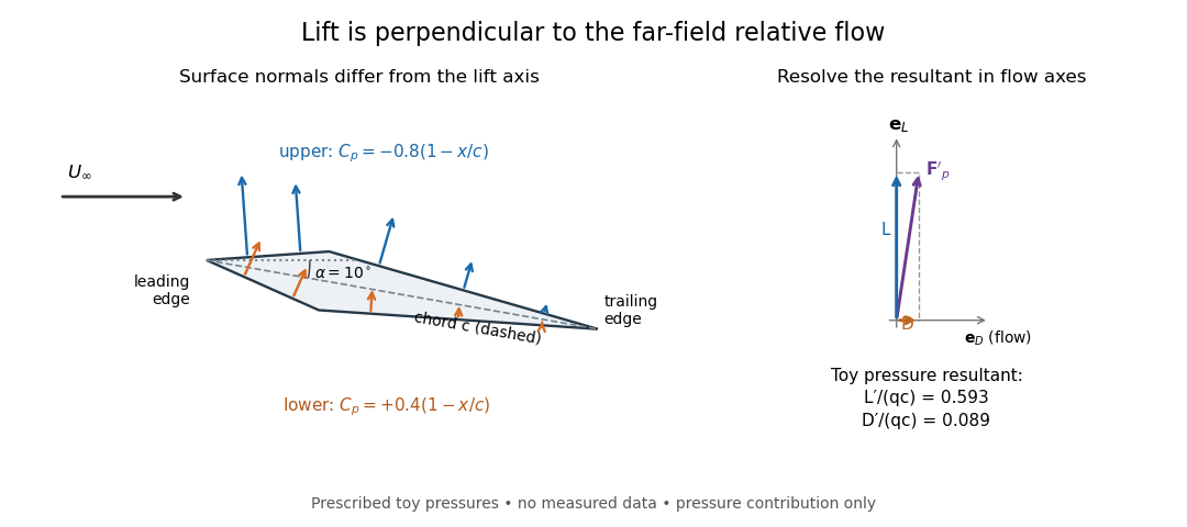
The lift coefficient isolates a useful scale. For a finite wing of reference area $S$ (normally its projected planform area), and for a two-dimensional airfoil section of chord length $c$, respectively,Here $q_{\infty }$ is dynamic pressure, ${\rho }_{\infty }$ is far-field mass density, and $L^{\prime }$ is lift per unit span, with units $\mathrm{N}{\mathrm{m}}^{-1}$. The signs of $C_L$ and $c_l$ follow the chosen lift axis. For stipulated values ${\rho }_{\infty }=1.20\mathrm{kg}{\mathrm{m}}^{-3}$, $U_{\infty }=20\mathrm{m}{\mathrm{s}}^{-1}$, $S=0.50{\mathrm{m}}^2$ and $C_L=0.60$, $q_{\infty }=240\mathrm{Pa}$ and $L=72\mathrm{N}$. Doubling $U_{\infty }$ gives four times the lift only if $C_L$ stays fixed: changes in Reynolds number, Mach number, surface condition or angle of attack can change it. ^[ref]

A motivating experiment is to compare two independently observed quantities: the lift registered by a force balance, and the lift inferred from surface pressures. A low-speed wind tunnel holds the model fixed while air passes it at adjustable speed; a calibrated balance measures forces, while small flush holes on both surfaces connect by tubing to differential-pressure sensors referenced to $p_{\infty }$. Iowa State's GA(W)-1 teaching model has $43$ taps around a $101\mathrm{mm}$ chord; its instructions give their coordinates and close the contour by repeating the first tap. A classroom comparison can combine this pressure-panel method with a balance on the same model; this is an experiment design, not a claim that those instructions report a combined measurement. ^{[ref] [ref]}

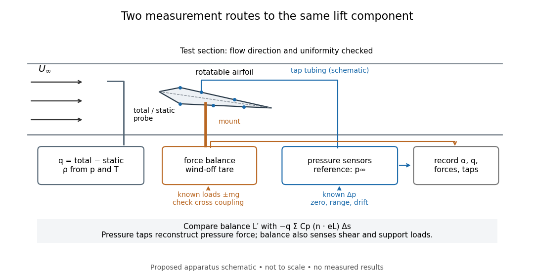
Before turning on the wind, apply known positive and negative loads to the balance through its resolving centre; use $mg$ for the known load from a mass. Record all balance channels during loading and unloading, including response to drag and torque loads, to detect cross coupling, hysteresis and zero drift. Record a wind-off tare at each model orientation so its weight does not become an aerodynamic lift reading. Map tunnel flow direction and uniformity, rather than using the fan setting as a speed measurement. Covert's MIT guide describes these calibration, tare and flow-survey requirements. ^[ref]

For each pressure channel, apply zero and several known pressure differences spanning the expected range; determine the voltage-to-pressure relation and recheck it after a run. Inspect tubing for leaks and blocked taps, and wait for readings to settle before averaging: tubing can delay a pressure signal. This calibration principle is used in NASA's electronically scanned pressure systems, where several applied calibration pressures determine each sensor's response and repeated calibration tracks drift. A simple pressure standard can instead use a liquid-column height difference and the hydrostatic pressure law. ^[ref]

Measure far-field static and total pressure outside the model's fluid wake; in low-speed incompressible flow their difference gives $q_{\infty }$ by the Bernoulli equation, so $U_{\infty }=\sqrt{2q_{\infty }/{\rho }_{\infty }}$. Record temperature and ambient pressure to determine mass density using the ideal gas law. At fixed $q_{\infty }$, step the angle of attack, repeat selected settings, and sweep back down to check reproducibility. Record balance lift, each tap's mean pressure, and fluctuation sizes. NASA describes pressure probes connected to differential transducers and emphasizes recording their reference pressure. ^[ref]

Convert each tap to a pressure coefficient $C_{p,i}=(p_i-p_{\infty })/q_{\infty }$. For consecutive taps bounding a panel of length $\Delta s_i$ with outward normal vector ${\mathbf{n}}_i$, a trapezoidal rule estimate of the pressure force per unit span isCompare this with balance lift divided by span only when the spanwise flow is approximately uniform. Agreement tests the pressure-resultant picture; disagreement calls for checking unresolved leading-edge pressure variations, skin shear stress, support loads and three-dimensional end effects before rejecting it. A force balance senses the total load, while taps alone reconstruct the pressure part. Tunnel walls and model blockage alter the effective flow and require corrections; end plates or a model extending between walls approximate two-dimensional flow but do not guarantee it. Record the Reynolds number and Mach number with the result, and do not interpret tunnel lift coefficients as universal wing data. ^{[ref] [ref]}

The signed lift divided by dynamic pressure times a stated reference area. For a two-dimensional airfoil, use $c_l=L^{\prime }/(q_{\infty }c)$ instead. Reference area and experimental flow conditions are part of the definition of a reported coefficient; see lift for a worked scale and a pressure/balance experiment.

Dynamic pressure is the bulk kinetic energy per unit volume associated with fluid motion at speed $U$ in a specified reference frame:Here $\rho =m/V$ is mass density. The word "pressure" identifies its units and its use as a pressure scale; $q$ is not an extra isotropic stress to add to the local static pressure in every surface traction. A stationary fluid can have large static pressure with $q=0$. Conversely, knowing $U$ and $\rho$ fixes $q$ without fixing static pressure. The definition remains useful in viscous fluid flow and compressible flow, even when the simplest Bernoulli equation is inapplicable. ^[ref]

For stipulated mass density ${\rho }_{\infty }=1.20\mathrm{kg}{\mathrm{m}}^{-3}$ and reference speed $U_{\infty }=20\mathrm{m}{\mathrm{s}}^{-1}$, $q_{\infty }=240\mathrm{Pa}$. At $40\mathrm{m}{\mathrm{s}}^{-1}$ with the same mass density, $q_{\infty }=960\mathrm{Pa}$. This quadratic scaling makes dynamic pressure a useful normalization for the lift coefficient, drag coefficient and pressure coefficient; it predicts four times a particular force only if its corresponding coefficient remains unchanged.

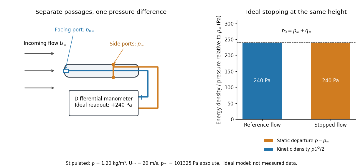
The connection with stagnation pressure requires hypotheses. For steady flow, constant mass density, inviscid flow, and gravity as the only body force, the Bernoulli equation gives, along one streamline,Here $p$ is static pressure, $g$ is gravitational acceleration, and $z$ is height. Bring that flow to rest without losses at the same height and the limiting static pressure is the stagnation pressure $p_0$:There must be no intervening pump supplying work or other energy input. Constancy along one streamline does not assert equal $B$ on all streamlines; irrotational flow in a connected region supplies that additional conclusion. Changing height requires retaining $\rho gz$. In compressible flow the stopping pressure difference generally differs from $\rho U^2/2$, and viscous dissipation can reduce recovered stagnation pressure. ^[ref]

A Pitot-static tube turns this relation into a measurement: its upstream-facing opening senses stagnation pressure, while separate side openings sample static pressure. Connect these to the positive and negative ports of a differential pressure transducer or manometer. Under the hypotheses above, the measured difference $\Delta p$ givesThus the stipulated $240\mathrm{Pa}$ and $1.20\mathrm{kg}{\mathrm{m}}^{-3}$ imply $20\mathrm{m}{\mathrm{s}}^{-1}$, not an independently measured speed. Align the probe with the incoming flow and keep its passages clear: blockage and pinched tubing invalidate the comparison. At very low speed, the difference can be smaller than instrument error; at high Mach number, compressibility and possibly a shock wave require a different reduction. ^[ref]

A useful control is differential-pressure calibration. For a digital manometer, zeroing establishes the reading at equal port pressures; it does not establish the gain away from zero. The manufacturer's Series 475 Handheld Digital Manometer: Specifications - Installation and Operating Instructions by Dwyer Instruments, Inc. directs the user to vent both ports to the atmosphere before zeroing. Its stated accuracy is a fraction of full scale, not of the reading, and depends on instrument temperature. Select a suitable range and record the instrument variant and units; the manual covers several ranges.^[ref]

An independent physical check can use a liquid-column manometer: apply a stable pressure difference to both instruments and compare the digital reading with the hydrostatic pressure inferred from the vertical level difference. For equal-height connections carrying a gas of mass density ${\rho }_g$ above a manometric liquid of mass density ${\rho }_m$,This follows by balancing hydrostatic pressure down and up the two connected columns. Use vertical height, even if a tube is inclined. Known mass densities, measured height and gravitational acceleration set the comparison scale. Check several differences across the working range and reverse the port connections to check the sign. This is a proposed independent check, not a claim that the cited teaching experiment performed a full instrument calibration. Recheck zero after reconnecting the sealed tubing; a zero adjustment alone cannot detect a blocked passage or an incorrect scale.

The pressure coefficient compares a local static pressure with a specified reference static pressure, using a fixed reference dynamic pressure:The reference mass density, speed, pressure and location must accompany a reported pressure coefficient. Keep the same $q_{\infty }$ throughout a surface distribution; replacing it by local $\rho U^2/2$ gives a different quantity and fails at a stagnation point. The definition itself requires neither Bernoulli's principle nor inviscid flow, so measured pressure coefficients remain useful when those idealizations fail.

Positive $C_p$ means $p>p_{\infty }$; zero means equality; negative $C_p$ means $p<p_{\infty }$. This sign does not specify the sign of absolute pressure. For stipulated $p_{\infty }=101325\mathrm{Pa}$ absolute and $q_{\infty }=240\mathrm{Pa}$, $C_p=-3$ gives $p=100605\mathrm{Pa}$ absolute: a $720\mathrm{Pa}$ deficit, not a negative absolute pressure. If $p_{\infty }$ equals atmospheric pressure, the numerator is gauge pressure; a wind tunnel's reference static pressure need not equal room atmospheric pressure. These are reference choices, not different physical pressures.

Under the same-height, constant-mass density $\rho ={\rho }_{\infty }$, steady flow and inviscid flow hypotheses of the Bernoulli equation, and with the same Bernoulli invariant as the reference flow,The first equation immediately gives the second after subtracting $p_{\infty }$ and dividing by $q_{\infty }$. Hence a lossless stagnation point has $C_p=1$, $U=U_{\infty }$ gives $C_p=0$, and $U=2U_{\infty }$ gives $C_p=-3$. For a real stationary wall satisfying the no-slip boundary condition, the velocity is zero right at the wall; inserting that wall velocity in an inviscid flow formula would wrongly predict $C_p=1$ everywhere. A thin boundary layer approximation instead relates the wall pressure to the outer-flow pressure and uses the outer velocity where the Bernoulli equation applies.

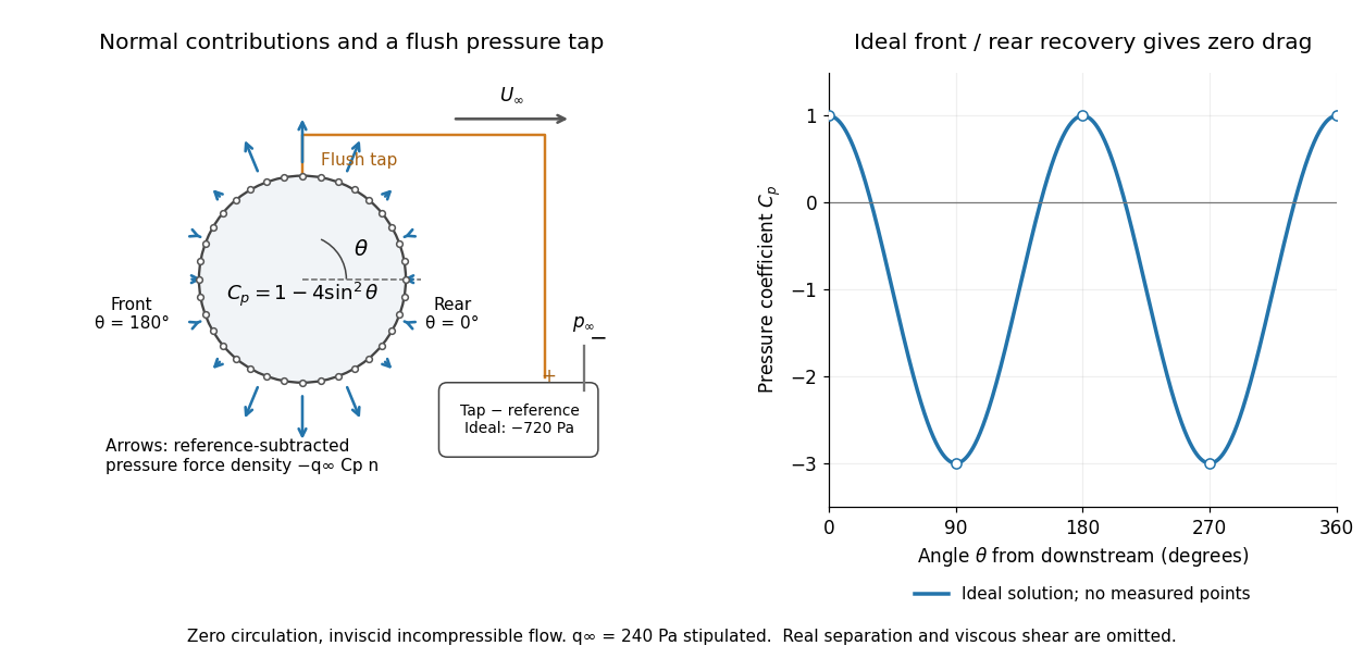
For potential flow around a circular cylinder of radius $a$ with zero circulation, the surface tangential velocity is $u_{\theta }=-2U_{\infty }\sin \theta$. Thus the ideal pressure coefficient isWith $\theta$ measured from downstream, the front is at $\pi$ and the rear at zero. Both ideal stagnation points have $C_p=1$, while the sides at $\pi /2$ and $3\pi /2$ have $C_p=-3$. This exact model is a useful baseline for an experiment; its complete rearward pressure recovery is not a prediction for a separated real fluid wake.

To obtain a force, integrate the local normal contributions with their directions. Let $\mathbf{n}$ be the unit normal vector from the body into the fluid and $\Sigma$ its closed wetted surface:The second equality removes a spatially constant reference pressure over the closed surface; it does not remove a nonuniform hydrostatic pressure or justify dropping the reference term on an isolated open patch. A negative $C_p$ contributes outwards in this reference-subtracted calculation, even though a positive absolute pressure still pushes inwards locally. Project ${\mathbf{F}}_p$ onto the chosen lift and drag directions. The full fluid force also includes ${\int }_{\Sigma }{\mathbf{\sigma }}_{\mathrm{visc}}\mathbf{n}dA$ from the viscous stress tensor, including tangential shear stress; pressure tapping does not measure that contribution.

For the two-dimensional cylinder, force per unit span follows from $dA=ad\theta$ per unit span and $\mathbf{n}=(\cos \theta ,\sin \theta )$:Substituting $C_p=1-4{\sin }^2\theta$ gives $(0,0)$: opposite points have identical pressure coefficients and opposite normal vectors. Zero drag despite a strongly nonuniform pressure is the instructive limitation associated with D'Alembert's paradox. Real viscosity, boundary layers and flow separation can prevent rearward pressure recovery and produce pressure drag. Thus the measured curve can test the model and estimate a pressure contribution without proving that total drag vanishes.

A motivating measurement is Virginia Tech's Experiment 3 - Flow Past a Circular Cylinder. Its open-jet wind tunnel holds a rotatable $140\mathrm{mm}$ cylinder with end plates and 36 one-millimetre pressure tappings at ten-degree intervals. A reference Pitot-static tube supplies $p_{0\infty }$ and $p_{\infty }$ to one digital manometer; a second connects a surface tap to its positive port and reference static pressure to its negative port. Record the simultaneous readings:The last equality uses the low-speed stopping relation, not an additional speed measurement. The manual requires sealed tubing and zero checks with the tunnel off. It also provides a water-column manometer: read each column's initial level, and subtract the independently measured reference-to-atmosphere pressure from the tap-to-atmosphere readings. Record tap positions after rotation. Compare the two instruments and check spanwise uniformity; end plates do not guarantee two-dimensional flow. ^[ref]

The inferential distinction matters: the manometers directly measure pressure differences, the ratio estimates pressure coefficients, and a surface integral estimates the pressure part of the force. Measure room absolute pressure and temperature if converting the reference difference to speed through the ideal gas law $\rho =p_{\mathrm{abs}}/(RT)$; use thermodynamic temperature in that equation. For force reconstruction, cover the complete contour and use numerical integration with the tap geometry. Finite tap spacing, unknown end effects, probe disturbance and fluctuations limit that reconstruction; tubes and instruments also average or delay changing pressures. Retain the signed raw readings, repeated readings and reference readings so that these limits can be assessed. A small reference difference magnifies any zero error in the ratio, rather than producing a reliably large $C_p$.

A small flush opening communicating the local surface static pressure through tubing to a manometer or pressure transducer. An upstream-facing Pitot tube instead brings incident flow to rest to measure stagnation pressure.