A particle accelerator increases the kinetic energy of charged particles through the work of an electric field. A single electric potential difference gives an energy gain of magnitude to a particle of electric charge crossing in the accelerating direction. Reusing a smaller electric potential difference many times can give a much larger final kinetic energy without requiring the whole apparatus to withstand the equivalent single voltage. A magnetic field can return the particles to the accelerating region: magnetic forces do no work, but they make repeated energy gains possible. The cyclotron turns this separation between bending and acceleration into a particularly elegant machine.
Measurements of beam properties such as intensity, position, transverse profile, bunch length, energy distribution, and losses. A diagnostic's calibration, bandwidth, and whether it intercepts the beam determine which changes can be inferred from its signal.
A nonintercepting circulating-beam current monitor that senses the beam's direct-current component through a magnetic core and feedback electronics. It is suitable for total stored intensity and beam lifetime measurements; zero-offset drift and calibration must be controlled. Bunch-resolved signals instead require an appropriate time-dependent pickup or current-transformer bandwidth.
The inverse fractional particle-loss rate of a stored beam. A constant rate gives ; density-dependent losses can make the instantaneous lifetime vary. At fixed revolution frequency, a calibrated beam-current measurement follows the same population decay, provided injection is absent or separately accounted for.
Intra-bunch Coulomb scattering can transfer transverse momentum into longitudinal momentum changes large enough to exceed a storage ring's accepted momentum range. This produces particle losses and a density-dependent contribution to the beam lifetime.
A driver excites charge-density oscillations in a plasma whose longitudinal electric field transfers energy to a trailing witness beam. Density fixes a characteristic plasma frequency and wavelength, while driver shape and loading determine the actual field and transfer efficiency.
A full pulse duration of roughly half a plasma period and a Gaussian rms duration of order the inverse plasma frequency are different conventions for a short resonant driver. Numerical estimates should state which width is meant. Maximum cold-wave fields also need not be produced by a specified driver with normalized amplitude below unity.
The cold nonrelativistic plasma field scale . It provides an order-of-magnitude density-gradient relation, not a complete nonlinear or relativistic wave-breaking criterion.
The ratio of the witness accelerating field to the driver decelerating field, with peak or loaded-field conventions stated. Under ideal common-length depletion, it also relates witness energy gain to driver energy loss.
The transverse transport of a charged-particle beam relative to a reference trajectory. Linear focusing gives betatron oscillations, described by Hill's equation and Courant-Snyder parameters; the beam envelope depends on its geometric emittance.
A linear paraxial map between transverse position and trajectory angle at two beamline locations. A drift of length has ; a focusing thin quadrupole has . Lossless uncoupled maps have determinant one. Repeated-cell bounded oscillatory motion requires ; at equality a Jordan block can still cause secular growth. This beam-optical map is distinct from a combinatorial transfer matrix.
For an initially parallel bundle passing through opposite equal thin-quadrupole strengths separated by , the two downstream focal distances differ as shown. Approximating the doublet by a common effective focal length discards that difference. A real common final focus requires additional incoming optical information or adjusted strengths.
A magnetic chicane's momentum-dependent path length does not specify a compression factor from initial length and marginal energy spread alone. A suitable longitudinal position-energy correlation is required. With zero correlation the variance above is minimized at , so such a chicane cannot shorten that ideal uncorrelated bunch. An imposed chirp and its uncorrelated residual determine the achievable minimum.
A lattice cell with two bending magnets whose dispersion and dispersion slope vanish at its boundaries. In an ideal identical-uniform-bend model with horizontal damping partition one, its minimum geometric emittance is , larger than the unconstrained theoretical minimum because of the achromatic boundary conditions.
The derivative of transverse betatron tune with respect to relative momentum error . For a thin-lens FODO cell with fixed quadrupole fields, natural cell chromaticity is on the stable phase-advance branch. Zero corrected chromaticity requires additional momentum-dependent focusing.
A beam intensity or photon flux per transverse phase-space volume, with any spectral bandwidth convention stated. In the far-from-diffraction-limited case with fixed flux and negligible dispersion contributions, brightness scales inversely with .
Photon source widths combine electron and diffraction widths in quadrature. At fixed optics, reducing electron emittance eventually has little effect when both radiation size and divergence dominate. This criterion differs from comparing emittances alone if the optical beta function is not matched to the diffraction ellipse.
A repeating focusing-drift-defocusing-drift lattice cell, with opposite quadrupole focusing in the two transverse planes. Stability and phase advance depend on focal strengths and separations.
The positive function and the displayed associated parameters describe a stable linear beam ellipse. A trajectory with invariant obeys and has phase advance . Writing gives ; the coefficient of is , not one.
The area occupied by a beam in transverse position-momentum or position-angle phase space, with a stated area or rms convention. Geometric emittance uses trajectory angle, while normalized emittance removes the ideal kinematic damping due to acceleration.
The phase-space area measure in the vertical transverse plane. If coupling is described by , changing the coupling and changing the natural emittance both alter its equilibrium value.
The phase-space area measure of the horizontal transverse beam distribution. With negligible dispersion and a specified optical function, it determines beam size and angular spread.
The equilibrium horizontal beam emittance set by synchrotron-radiation excitation and damping in an uncoupled storage ring. The radiation-integral relation is ; similar cell optics give a cubic dependence on bending angle.
The geometric emittance multiplied by the relativistic velocity and Lorentz factor. For paraxial acceleration without dilution, this is proportional to transverse canonical phase-space area and remains constant. Thus geometric emittance decreases approximately as inverse beam momentum.
For a centered beam, the displayed rms area in coordinates. A matched beam has , where is one of the Courant-Snyder parameters. Under ideal acceleration, adiabatic damping of geometric emittance decreases this area even when the canonical phase-space area is preserved.
For slowly accelerated paraxial motion, decreases as longitudinal momentum grows while transverse canonical phase-space area is conserved. The normalized emittance stays constant in the ideal limit, so the geometric emittance scales inversely with longitudinal momentum. This is kinematic damping rather than dissipation of canonical area.
Small transverse oscillation about an accelerator's reference orbit. In a linear periodic lattice the displacement obeys Hill's equation .
For rms geometric beam emittance , the transverse beam variance is . At a beam waist, the angular variance is . Reducing both transverse amplitude functions by a factor at fixed emittances increases the ideal head-on collider luminosity by ; practical finite-bunch-length and crossing-angle effects can limit this gain.
Alternating focusing and defocusing quadrupole magnets, separated by drifts, can give stable net focusing in both transverse planes. Stability depends on the full transfer matrix of the lattice cell, not on the sign of one magnet alone.
A magnet whose transverse field varies linearly with displacement. Its Lorentz force focuses a charged-particle beam in one transverse plane and defocuses it in the other. Oppositely oriented elements provide alternating-gradient focusing.
At fixed gradient and magnet length, the signed thin-lens focal length is proportional to particle momentum. For total energy error , differentiating gives . The ultrarelativistic result is to first order. If energy means kinetic energy instead, the coefficient is .
An element of the strong focusing system near a collider interaction point. It helps form a small transverse beam waist there, matched to the surrounding periodic lattice. Small collision-point beta functions generally imply large envelopes and strong chromatic effects in nearby magnets.
A particle accelerator that brings counterpropagating electron and Positron beams into collision. The known initial four-momentum and tunable center-of-mass energy make resonance scans and missing-energy measurements possible.
A CERN electron–positron collider. Its higher-energy operation made W-pair production available for measurements of electroweak triple gauge couplings.
- Evidence for light-by-light scattering in heavy-ion collisions with the ATLAS detector at the LHC by ATLAS Collaboration
- Search for squarks and gluinos with the ATLAS detector in final states with jets and missing transverse momentum using 4.7 fb^-1 of sqrt(s) = 7 TeV proton-proton collision data by ATLAS Collaboration
A circular particle accelerator with bending fields and accelerating fields varied in coordination with the increasing beam momentum.
The integer number of radio-frequency cycles per revolution of a synchronous particle in a circular accelerator. It fixes and the number of RF buckets around the ring. It is unrelated to an arithmetic harmonic number .
The Brookhaven proton synchrotron used for the Lederman-Schwartz-Steinberger two-neutrino beam experiment.
A particle accelerator in which a beam gains kinetic energy along a substantially straight sequence of accelerating structures.
A collider whose main beams are accelerated along opposing linear beamlines and brought into collision without returning repeatedly around a storage ring. Sources, beam conditioning, final focus, extraction, and dumps are essential parts of the layout, as well as the main accelerating structures.
A proposed electron–positron linear collider using normal-conducting RF structures powered through a separate drive-beam deceleration system. The 2012 conceptual design studied multi-TeV operation and lower-energy stages; its TeV design used approximately MV/m main-linac gradients. Historical design targets should be distinguished from later staging revisions and from operating measurements. [ref]
https://cds.cern.ch/record/1500095. CLIC Conceptual Design Report, CERN-2012-007, abstract and accelerator concept
A proposed electron–positron linear collider based on superconducting RF acceleration. The 2007 reference design relevant to an exam-era comparison targeted GeV centre-of-mass energy and peak collider luminosity , with approximately km total footprint. These are historical design parameters, not achieved machine performance. [ref]
A cyclotron repeatedly passes ions through an alternating electric field between two hollow electrodes called cyclotron dees. A nearly uniform magnetic field perpendicular to their plane bends the charged particles back toward the gap. Inside each cyclotron dee, ideal shielding suppresses the accelerating electric field, so each segment is a constant-speed circular motion. The next gap crossing increases the speed and the radius of curvature. The complete path consists of connected, progressively larger arcs, rather than one circle or a smooth spiral with continuous acceleration everywhere.
The striking feature is a timing cancellation: the longer arc traveled by a faster particle takes the same time. This cyclotron resonance condition lets one fixed radio frequency accelerate many successive gap crossings. The following construction and cyclotron energy and orbit radius example describe an ideal model; the Lawrence-Livingston cyclotron experiment explains what the builders actually measured.
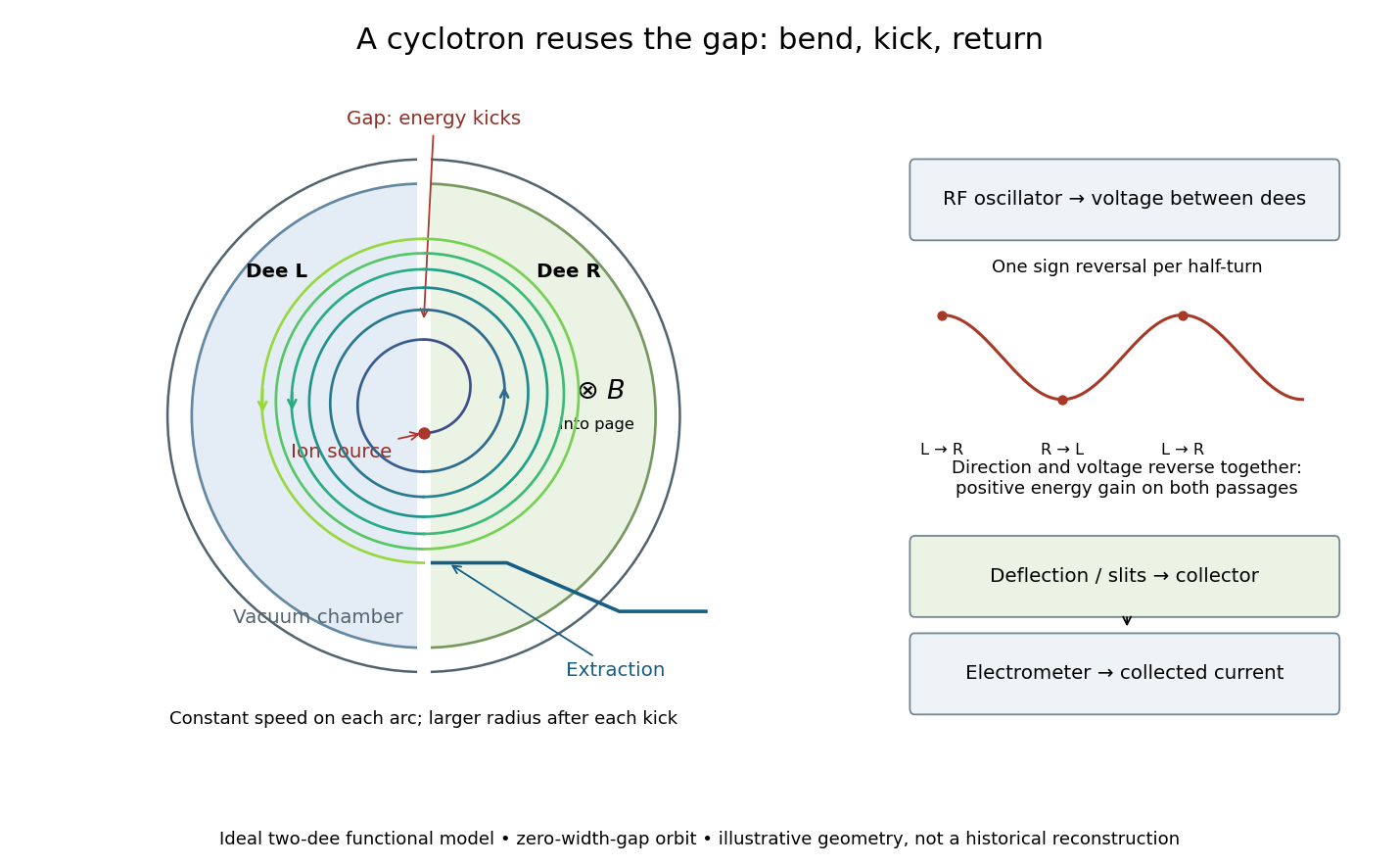

A hollow D-shaped electrode that shields a circulating ion from the accelerating electric field during one half-turn. Two opposed cyclotron dees provide two shielded regions separated by a gap; their electric potential difference alternates. The vacuum reduces collisions with residual gas. An ion source supplies particles near the center, and an extraction system directs an outer orbit toward a particle detector or target. Useful electric current depends on retaining particles near the median plane and delivering them to the outlet, as well as on increasing their kinetic energy.
Take an ion of mass and electric charge , with velocity perpendicular to a uniform magnetic field of magnitude . In the classical mechanics limit, the Lorentz force provides the centripetal acceleration:Here is the local radius of curvature and is the cyclotron frequency, expressed as an angular frequency. A half-turn takesIncreasing speed increases the path length in exactly the same proportion. Drive the gap at angular frequency , or ordinary frequency . In each half-turn the gap electric field reverses once, just as the particle reverses its direction of passage through the gap. The particle therefore receives two accelerating kicks per complete turn, using one oscillation per complete turn. This is the fundamental resonance; transit time through the gap and departures from a uniform magnetic field have been neglected.
Define as the electric potential drop along the particle's passage. If the electric field changes negligibly during that short crossing, the work givesThe sign matters: a positive ion gains kinetic energy while going to lower electric potential; a negative ion needs the opposite drop. A fixed-sign field would accelerate on one crossing and decelerate on the next. The alternating field must reverse before the particle comes back.
For a fixed electric charge sign and circulation direction, absorb this alternating crossing direction into the definition of the arrival phase . If is the peak electric potential difference across the whole gap, rather than the amplitude of either electrode relative to ground, a thin-gap model isArrival at gives the largest accelerating kick; gives a positive kick. Arrival at gives deceleration. For an ideal classical particle initially on crest, the cyclotron resonance condition keeps successive arrival phases equal. It does not automatically bring an initially mistimed particle onto crest.
Combining with the classical kinetic energy givesHere denotes kinetic energy, not relativistic total energy. At fixed magnetic field, twice the final radius allows four times the classical kinetic energy. At fixed final kinetic energy, a larger accelerating gap voltage reduces the number of crossings needed, but does not change the required orbit radius.
For an illustrative proton with and peak gap voltage , take negligible injection kinetic energy, on-crest kicks, a zero-width gap, and no losses. Each crossing adds , so crossings give , using electronvolts. With and ,The th kick arrives after intervening half-turns, about after the first kick in this idealization. The final two curvature radii differ by . That difference is a curvature-radius increment, not a general formula for separation of real extracted turns: successive arc centers shift, and extraction also depends on focusing and the gap geometry. These chosen settings are a calculation, not historical measurements.
Ernest Orlando Lawrence and Milton Stanley Livingston reported repeated ion acceleration in 1932. Their evacuated brass chamber used one driven hollow cyclotron dee; the grounded box and slotted divider supplied the other electrode. Filament electrons ionized hydrogen near the gap. A perpendicular magnetic field bent the ions; a high-frequency oscillator drove the gap. Deflecting plates and slits selected particles for a Faraday cup, read by an electrometer.[ref]
The Production of High Speed Light Ions Without the Use of High Voltages by Ernest Orlando Lawrence and Milton Stanley Livingston. Lawrence and Livingston, 1932, pp. 25–28, Figs. 2–4: actual accelerating electrode, source, collector and oscillator
Scanning the magnetic field produced narrow resonance peaks. The optimum deflecting voltage tracked the kinetic energy predicted from field and orbit radius, supporting the reported protons. Source width and slit geometry limited this check; it was not a direct energy measurement of every particle.[ref]
The Production of High Speed Light Ions Without the Use of High Voltages by Ernest Orlando Lawrence and Milton Stanley Livingston. pp. 31–33, Figs. 7–9: resonance scans, field and wavelength measurements, deflection-voltage energy check and geometric uncertainty; p. 19: maximum reported proton energy
This combination distinguishes producing a circulating electric current from establishing its kinetic energy. The electrometer measures collected electric charge per unit time; it cannot by itself tell whether the collected particles are fast. The separate deflection selection supplies a speed-dependent test. Agreement of two consequences of the model, the cyclotron resonance condition and the cyclotron energy and orbit radius relation, makes the inference stronger than either a current signal or a predicted orbit alone.
Milton Stanley Livingston built the early cyclotrons with Ernest Orlando Lawrence; the 1939 Nobel Prize in Physics went to Ernest Orlando Lawrence. His lecture, The evolution of the cyclotron, was delivered on 11 December 1951.[ref]
More Timelines by Lawrence Livermore National Laboratory. Ernest Lawrence entry: 1939 prize and delayed lecture on 11 December 1951
[ref]M. Stanley Livingston by Fermilab. M. Stanley Livingston: co-inventor of the cyclotron and early Berkeley work
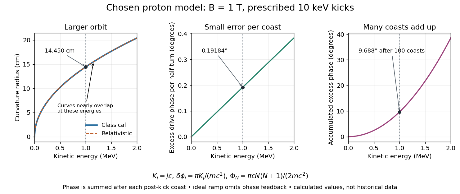
At larger kinetic energy, special relativity changes the relation between momentum and velocity. With the invariant mass, the Lorentz factor is , and a relativistic cyclotron orbit in a fixed uniform magnetic field satisfiesThe cyclotron frequency decreases as the kinetic energy increases. If the drive stays at the classical value , the half-turn time is . During it the drive advances through rather than radians. Its excess phase per half-turn is thereforeEven a small fractional frequency mismatch accumulates across many turns. A particle eventually reaches a weak or decelerating gap phase, so the classical fixed-field, fixed-frequency design has a practical kinetic energy limit. The limit depends on the kick size and acceptable accumulated phase error, rather than one universal cutoff energy. Changing drive frequency or shaping the magnetic field can restore synchronism; the argument does not forbid relativistic circular accelerators.
For the illustrative proton at , : the frequency is lower by about , and the next half-turn adds about of drive phase excess. To see cumulative sensitivity, prescribe an ideal ramp with and sum the errors of the first coasts after kicks:This gives after the coast following kick ; the arrival at kick instead has . The prescribed ramp diagnoses detuning but does not feed the resulting phase error back into the kicks. A self-consistent thin-gap model uses the cyclotron gap energy gain with , then advances the phase with the new kinetic energy during the following coast.

An electrostatic accelerator gives a charged particle kinetic energy by taking it through a sustained electric potential difference. Its ion source, accelerating tube and target form a particularly direct chain: prepare a charge, let an electric field do work, and measure what arrives or what the target emits. A vacuum reduces collisions with gas before the beam reaches its target. The Cockcroft-Walton generator supplies the potential by accumulating electric charge on capacitors.
For a fixed electric charge , a time-independent electric potential and negligible collisions or radiation losses, conservation of energy givesHere is the signed potential drop along the trajectory. A proton starting nearly at rest at and arriving at ground gains : a chosen gives , by the definition of the electronvolt. Several intermediate electrodes can distribute that drop along a tube, but the gains telescope to the same endpoint difference. Passing through more electrodes does not multiply the available kinetic energy beyond .
This is the distinction from a cyclotron. In a static electric field, a closed trip gives zero net work. A cyclotron changes the gap electric field between successive visits, so correctly timed particles repeatedly gain kinetic energy. Its limit involves the cyclotron resonance condition and relativistic detuning of a cyclotron; a single-pass electrostatic accelerator instead requires the full accelerating electric potential difference to be sustained at once. Neither machine's beam energy by itself specifies the energy released by a nuclear reaction.
A voltage multiplier made of rectifiers and capacitors that transfers electric charge from an alternating supply into a series stack of stored electric potential differences. The rectifiers allow charge transfer during selected portions of the cycle; the capacitors retain charge between transfers. The supply continually replaces charge removed by the load. Multiplication of voltage does not multiply energy: the input must supply the output power and losses.
In his 1951 lecture The Artificial Production of Fast Particles, Ernest Thomas Sinton Walton describes the fourfold multiplier's series storage capacitors and alternating transfer capacitor in Fig. 2, p. 190. This is a mechanism for producing a nearly steady accelerating potential from an alternating input.[ref]
The Artificial Production of Fast Particles by Ernest Thomas Sinton Walton. The Artificial Production of Fast Particles, lecture delivered 11 December 1951, p. 190, Fig. 2: storage and transfer capacitors; indexed primary text inspected
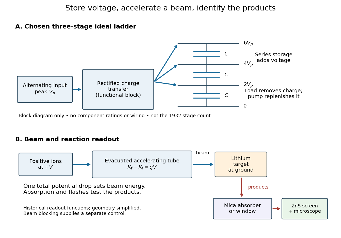
Voltage accumulation and particle acceleration are different steps
. Original functional diagram. Three ideal storage stages illustrate a chosen multiplier model; charge transfer is shown as a functional block rather than a wiring diagram. The beam crosses one total potential drop. The lower chain summarizes the lithium experiment's target and scintillation readout, not the geometry or stage count of the 1932 apparatus. Details.
Define a stage as one storage increment of , with the alternating input's peak electric potential difference relative to its reference, not its peak-to-peak value. Assume ideal rectifiers, no load, no leakage or stray capacitance, a stiff alternating source and enough cycles to reach equilibrium. For such stages,The factor two follows from adding the input's next opposite excursion to an already stored peak. The subsequent series increments add. This ideal argument concerns equilibrium voltage; it supplies neither the charge-up time nor the useful load electric current.
To isolate the effect of drawing charge, consider the following original reservoir model. Each storage stage has equal capacitance ; a constant output electric current removes between replenishment events of frequency . Every series reservoir loses this charge, hence its voltage falls by per interval. Suppose replenishment removes a fixed fraction of each reservoir's accumulated deficit, with . This is an explicit phenomenological pump rule, not a solution of a particular multiplier's rectifier network. If is the deficit immediately after event , thenHere and are the equilibrium deficits just after and just before replenishment. Linear discharge between events gives the average output and peak-to-peak variationFor chosen dimensionless settings , and , the output varies between and , averaging , instead of the unloaded . Starting with zero deficit, the recurrence approaches equilibrium geometrically with factor . Taking recovers the ideal ladder; increasing or reduces droop in this model. As , effective replenishment fails and the small-deficit assumption fails too.
Real multiplier stages have unequal charge-transfer burdens; their mean deficits need not be equal and depend on topology, input impedance and parasitic capacitance. Thus this reservoir model explains droop and voltage variation without claiming their exact dependence on stage count for a real Cockcroft-Walton generator. In particular, adding more stages cannot be judged solely by the unloaded . For a beam sampling a slowly varying output, the electrostatic acceleration energy gain follows that instantaneous potential drop, so voltage variation also produces a spread of beam kinetic energies.
In 1932 John Douglas Cockcroft and Ernest Thomas Sinton Walton accelerated hydrogen ions from a discharge source through an evacuated tube onto lithium at . A side-facing zinc sulfide screen, viewed by microscope, showed particle scintillations. Mica stopped scattered protons; switching off or blocking the beam removed the flashes. An external screen allowed absorption-range measurements.[ref]
Experiments with High Velocity Positive Ions. II. The Disintegration of Elements by High Velocity Protons by John Douglas Cockcroft and Ernest Thomas Sinton Walton. Experiments with High Velocity Positive Ions. II. The Disintegration of Elements by High Velocity Protons, 1932, pp. 230–232, sections 2–3, Fig. 1; primary text inspected in the Scribd transcription
Magnetic deflection checked voltage calibration. Opposite screens and independent observers found excess coincidences for a thin lithium target, supporting paired alpha particle emission; geometry and screen efficiency limited detection.[ref]
Experiments with High Velocity Positive Ions. II. The Disintegration of Elements by High Velocity Protons by John Douglas Cockcroft and Ernest Thomas Sinton Walton. pp. 231, 237–238, section 4, Figs. 5–6: corrected voltage calibration, paired screens and random-coincidence comparison
John Douglas Cockcroft's 1951 lecture recalls detection at and an absorption range about , then refined alpha particle energies about each. He places the work under Ernest Rutherford's direction. The inferred nuclear reaction was lithium-7 plus a proton producing two alpha particles.[ref]
Experiments on the interaction of high-speed nucleons with atomic nuclei by John Douglas Cockcroft. Experiments on the interaction of high-speed nucleons with atomic nuclei, lecture delivered 11 December 1951, pp. 167–170, Figs. 2–4; primary text inspected in the Scribd transcription
The logic has several independent links. Beam blocking tests whether the flashes depend on bombardment. An absorber tests whether scattered beam particles could reach the screen. A particle range tests product identity and kinetic energy, while coincidences test whether two products belong to one event. These tests support a reaction interpretation jointly; counting flashes alone is not an isotope identification, and a range-to-energy conversion needs calibration. The lithium proton reaction energy below is a modern calculation, separate from those historical measurements.
The nuclear reactionconserves electric charge and total nucleon count: and . Its nuclear reaction Q-value is the initial minus final rest energy. It is additional to the incoming beam kinetic energy; the accelerator triggers a rearrangement whose products can carry much more kinetic energy than the incident proton.
Use one consistent set of neutral-atom isotope masses, in unified atomic mass units, from the National Institute of Standards and Technology:These are isotope masses, not element-averaged atomic weights.[ref]
Atomic Weights and Isotopic Compositions for All Elements by National Institute of Standards and Technology. Atomic Weights and Isotopic Compositions for All Elements, entries atomic number 1 mass number 1; atomic number 2 mass number 4; atomic number 3 mass number 7
With ,[ref]CODATA recommended values of the fundamental physical constants: 2022 by National Institute of Standards and Technology. CODATA recommended values of the fundamental physical constants: 2022, atomic mass constant, energy equivalent in MeV
The four electron rest masses cancel between sides. Differences of total electronic binding energies do not cancel exactly: this atomic-mass result approximates the bare-nucleus nuclear reaction Q-value at the displayed scale, not at arbitrary precision. No mixture of rounded nuclear binding energies is needed. At chosen incident kinetic energy on a stationary target, the two outgoing alpha particles together carry approximately before losses in the target and detector window.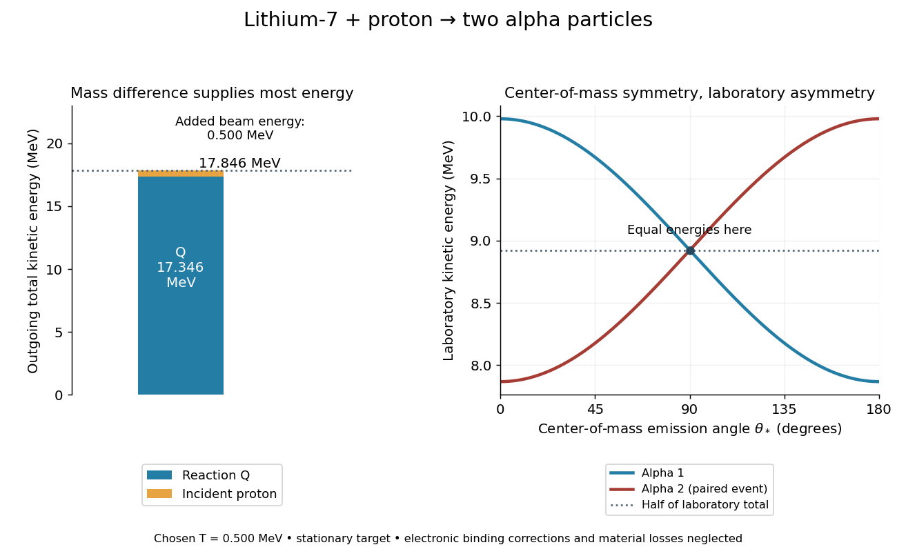

Equal product masses imply equal kinetic energies and opposite momenta in the center of mass frame. The laboratory frame has nonzero initial momentum because the proton is moving. Conservation of momentum therefore forbids the two laboratory momenta from always being equal and opposite. The products are equal in laboratory kinetic energy only for particular emission directions, not for every event.
An exact two-body calculation makes this distinction quantitative. Write , , , and for incident kinetic energy. Express every quantity below in the same energy units; is momentum times the speed of light. For a stationary target,Here is the center-of-mass energy, and is the center-of-mass speed divided by the speed of light. Each outgoing alpha particle has center-of-mass total energy and momentum-times- magnitude . A Lorentz transformation gives the paired laboratory kinetic energies, with measured from the incident beam in the center of mass frame:Their sum is independent of and equals . Their difference is ; the symmetry belongs to the product interchange and the center of mass frame.
For the chosen model, subtract electron rest masses from each neutral-atom mass, neglect electronic binding energies, and use .[ref]
CODATA recommended values of the fundamental physical constants: 2022 by National Institute of Standards and Technology. CODATA 2022 wall chart, electron mass, energy equivalent in MeV
At , the paired laboratory kinetic energies are approximately and ; at both are approximately . In the latter case both products have a forward laboratory momentum component, so even equal laboratory kinetic energies do not imply back-to-back laboratory trajectories. A real thick target and finite detector acceptance would broaden or select these ideal kinematic possibilities.An accelerator technician who contributed to the development of the hydrogen bubble chamber.[ref]
https://escholarship.org/content/qt2fw5366k/qt2fw5366k.pdf. Alvarez lecture, UCRL-18696, printed pp. 13–15: John Wood's work as an accelerator technician and early hydrogen-chamber development
The Super Proton-Antiproton Synchrotron used the converted SPS ring for counterrotating proton and antiproton beams. In the discovery running, two beams provided , unlike a stationary-target collision at the same incident energy. Antiproton production, accumulation and stochastic cooling supplied the collisions used in the W and Z discovery experiments.[ref]
Experimental Observation of the Intermediate Vector Bosons W+, W− and Z0 by Carlo Rubbia. Section 3, printed p.247 and Fig.5: counterrotating beams, accumulation and SPS conversion
Why can opposite electric charges share the bending magnets? Reversing both and velocity leaves the Lorentz force unchanged at a given point. Both circulating species can therefore bend toward the same ring center in the same magnetic field, with equal magnetic rigidity magnitudes. This argument explains the bending geometry; actual injection, focusing, timed acceleration and collisions still require a complete particle accelerator system.
Beam cooling reduces random deviations around a beam's reference motion, such as its momentum spread and transverse spread. A highly energetic beam can be cool in this sense: its large common directed kinetic energy is distinct from the spread. Concentrating the occupied phase space helps accumulated particles fit the next machine's acceptance. Stochastic cooling achieves this through measured beam fluctuations and feedback control.
Cooling an ion beam through Coulomb interactions with a co-moving low-spread electron beam. Friction reduces ion motion relative to the electron guiding flow while diffusion and external heating determine the eventual equilibrium.
Strong longitudinal magnetic guidance can average rapid electron gyro-motion during relevant ion-electron interactions. The effective ion equilibrium scale can then be much lower than the transverse electron gyro-temperature, subject to gyroradius, collision-scale and beam-quality limits.
Simon van der Meer's stochastic cooling uses measured beam fluctuations, a pick-up, amplifier and timed kicker. Finite samples supply the signal; other particles and electronic noise contribute unwanted kicks. Delay and oscillation phase must make the correction oppose the sampled deviation.[ref]
This active system dissipates energy; it is no one-particle Maxwell's demon individually tracking antiprotons. The stochastic cooling variance model isolates the tradeoff.
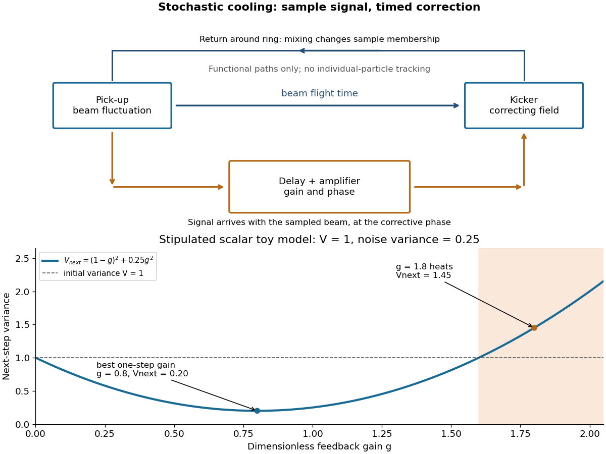

Beam mixing changes sample membership between turns through revolution-time differences. Repeatedly correlated samples and thermal noise limit stochastic cooling.[ref]
Stochastic Cooling and the Accumulation of Antiprotons by Simon van der Meer. Section 5, p.295, Mixing and thermal noise, Eqs.(3)–(4)
Fresh samples help across turns; losing pick-up–kicker correlation hurts. Useful feedback gain therefore depends on bandwidth, delay, beam dynamics and signal-to-noise ratio.
Let be a centered scalar beam-deviation coordinate in a deliberately controlled toy model. Let the readout be , where the centered measurement noise has variance and is independent of and of earlier noise. Stipulate a correctly timed correction of strength : . This scalar observation is a teaching surrogate, not a claim that real cooling measures each particle. From variance additivity for independent random variables,For fixed current and , differentiate the next-step variance with respect to feedback gain:The unique one-step minimizing feedback gain and resulting variance areThe noisier the readout relative to the current spread, the smaller the useful correction. The exact one-step cooling condition follows by subtraction:Thus excessive positive feedback gain heats this model. The threshold depends on the current variance: a gain that initially cools can later heat if the beam has become narrower or the noise has grown.
For chosen dimensionless and , gives . Taking instead gives , larger than the initial spread. Holding fixed givesso the variance approaches the nonzero noise floor . More generally, for the fixed-gain limit is . This long-run stability condition differs from the condition for cooling the current beam on the very next step.
If the toy feedback gain is recomputed after every step and , the reciprocal recurrence is even simpler:With the chosen inputs, . This ideal model has no additional diffusion, finite observation time or lost correlation; its indefinitely falling spread is not a prediction for an operating storage ring.
To expose the missing physics mathematically, replace by an arbitrary centered sample signal . Defining and givesUnwanted contributions from other particles or electronics can enlarge without increasing useful ; poor timing or lost correlation can reduce or even reverse its sign. This is why real stochastic cooling needs measured beam fluctuations, appropriate beam mixing and correctly phased feedback control, rather than an imagined catalogue of individual particle positions.
An instrument that compares quantities through their mechanical effects, historically central to quantitative chemistry. Material accounting requires including all relevant substances, not merely weighing a visible solid.
A particle beam dominated by neutrinos. Accelerator beams can use particle decay of focused charged pions and kaons, followed by shielding that suppresses other beam components.
A decay tunnel provides a low-density flight region where selected unstable particles decay before remaining charged particles are removed or absorbed. For a pion-produced neutrino beam, its length balances pion decay probability against backgrounds from longer-lived daughters.
A magnetic horn uses a pulsed magnetic field around a high-current conductor to focus charged secondary pions and kaons of a selected sign. Their decays then create a directed neutrino beam. The field acts on the charged parents, not on the neutral neutrinos.
Here particle flux means the number of particles crossing a surface per unit area and unit time, with the area taken perpendicular to the incident particle beam. Multiplying by the target interaction cross section gives an event rate per target particle in the ideal independent-target model.
The particle flux of neutrinos through a specified surface; an incident-energy distribution may also be specified.
A stream of positive ions in a gas discharge. Historical canal rays pass through holes in the cathode; collisions can also produce moving neutral chemical atoms.
A molecular beam also includes a stream of chemical atoms, then called an atomic beam. An oven supplies particles; aligned slits restrict their directions, and a vacuum limits subsequent collisions. Narrowing the directions does not by itself make every particle's speed equal. This gives a useful separation of tasks: prepare a path, select or measure speed, apply an interaction, and read the resulting particle counts or deflection.
The advantage is unusually tangible. A magnetic field can separate spin components in the Stern-Gerlach experiment; even gravity can sort a beam by flight time. The effusive beam speed distribution explains which particles leave the source, while gravity deflection of an atomic beam explains how that distribution becomes a pattern on a detector.
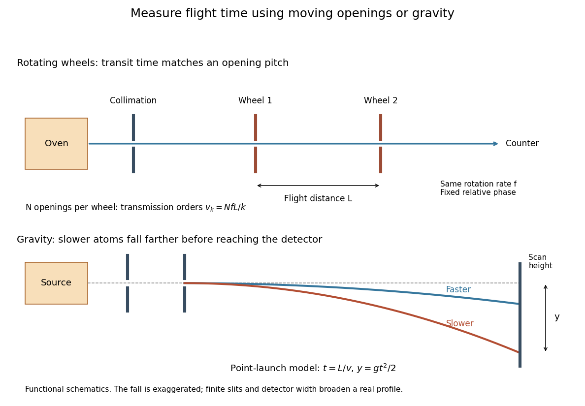

In 1911, Louis Dunoyer de Segonzac formed a sodium beam in vacuum and collected a deposit on a surface cooled with liquid air. Its shape agreed with straight paths through the slits.[ref]
The Method of Molecular Rays by Otto Stern. The method of molecular rays, lecture 12 December 1946, pp. 8–9: Dunoyer's sodium beam, collimation and cooled collector
A deposit tests the geometry of the surviving paths. A clock or a calibrated deflection is needed to turn their travel into a speed measurement.Which speed distribution does an arrival counter measure? Suppose an equilibrium, nonrelativistic ideal gas escapes by effusion through a thin opening into vacuum. The opening is small compared with the mean free path; the reservoir remains at temperature . Let denote its normalized Maxwell speed distribution, with mass and :At a given direction toward the opening, the number crossing per unit time is proportional to the normal component . Integrating over a fixed accepted cone contributes an angular factor independent of . Thus the normalized probability density function for speeds among arriving particles isIts integral is one because . The reservoir mode is ; the arrival mode is . Faster particles get more opportunities to cross the opening. This is a selection effect, not heating after emission.
Specify the observable before applying the formula. An instantaneous count in a fixed segment of the beam weights the arrival flux by the time spent there, proportional to ; in this ideal model its normalized speed law returns to . A detector's speed-dependent efficiency, source collisions or a velocity selector changes the arriving law again. Counting arrivals and counting particles currently present are different measurements.
Otto Stern's lecture describes two co-rotating toothed wheels: transit between them must match an advance between openings. He explicitly distinguishes this method from the first historical speed measurement.[ref]
The Method of Molecular Rays by Otto Stern. The method of molecular rays, lecture 12 December 1946, p. 9: rotating-wheel timing, transmission and limited accuracy
For an idealized example, let aligned wheels have equally spaced openings, separation , and rotation rate in revolutions per second. A particle with constant longitudinal speed takes between them. The second wheel advances through revolutions; transmission peaks when that advance is an integer number of opening pitches:With chosen , and , the first two orders select and . A second transmission maximum therefore need not represent a second source temperature. Finite opening widths admit speed intervals around each order, and an additional measurement is needed to distinguish orders. The ideal expression assumes negligible acceleration and constant rotation rate during a flight, with a fixed relative phase between the wheels.
Immanuel Estermann, O. C. Simpson and Otto Stern used gravitational deflection to measure atomic speeds. Stern describes scanning a hot-wire surface ionization detector through a cesium beam and recording ion electric current.[ref]
The Method of Molecular Rays by Otto Stern. The method of molecular rays, lecture 12 December 1946, pp. 9–11: collaborators, falling beam and ion-current readout
Their 1947 paper reports potassium and cesium beams; a deficit of slow arrivals increased with oven pressure, supporting a source-slit collision explanation.[ref]The Free Fall of Atoms and the Measurement of the Velocity Distribution in a Molecular Beam of Cesium Atoms by Immanuel Estermann, Oliver Cecil Simpson, and Otto Stern. Estermann, Simpson and Stern, Physical Review 71 (15 February 1947), p. 238, abstract: gravity deflection, modified Maxwellian distribution and pressure-dependent slow-atom deficit
First consider an original point-launch model, with horizontal speed , zero initial vertical velocity, flight distance , and uniform gravitational acceleration . Downward displacement follows from flight time :Slow particles fall farther. However, a detector scan counts arrivals per interval of height, not per interval of speed. Change of variables for probability densities supplies the Jacobian determinant:Here denotes the effusive beam speed distribution; the unadorned constant in denotes gravitational acceleration. The integral of is one: substituting reduces it to . Its mode is . Simply mapping the most probable arrival speed into a fall distance instead gives . The peaks differ because equal height bins cover unequal speed intervals.
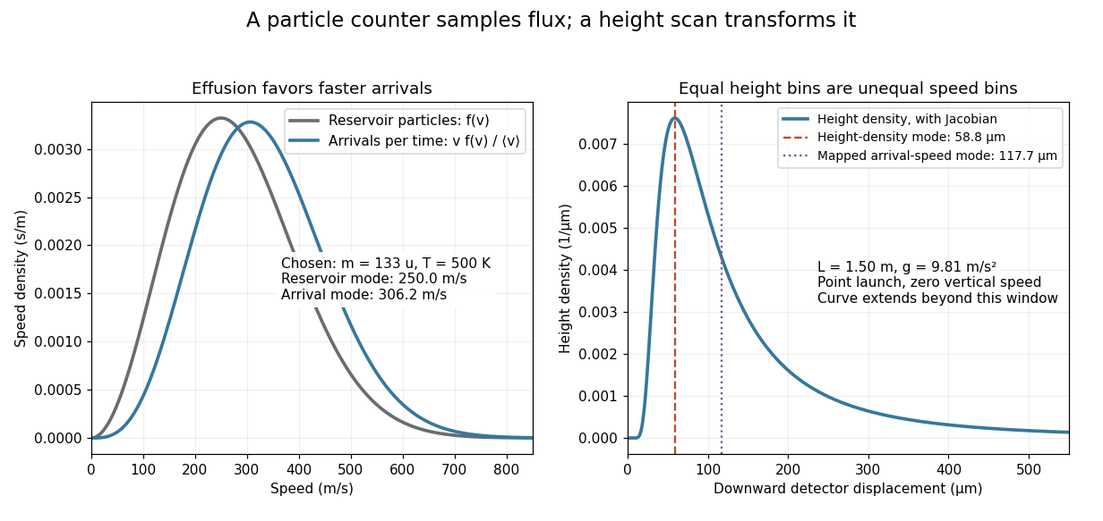
Effusion changes the arrival speed distribution, and a detector-height scan requires another Jacobian determinant
. Original calculated distributions with chosen , , and . These are not historical measurements. Details.
For those chosen parameters, , so the detector-height probability density peaks near . A detector covering only accepts the fractionAt this is about , even before allowing for imperfect detection. Discarding the remainder changes the observed normalization.
Real slits transmit a range of launch heights and vertical velocities. Their geometrical response must be combined with the gravitational deflection and detector width; the point-launch formula is not an exact reduction of the historical apparatus. In the point-launch model, an initial vertical velocity would add to . Source collisions, detector efficiency and alignment can also distort a profile. Varying oven pressure helps distinguish such source losses from an incorrect thermal distribution; inferring a source temperature from the peak alone ignores both selection and the detector's coordinate transformation.
A directed stream of chemical atoms, such as the neutral silver stream in the Stern-Gerlach experiment.
A load cell is a calibrated device for measuring force. In a tensile modulus experiment its output supplies the axial load used to calculate engineering stress.
An X-ray observatory used for high-resolution imaging and spectroscopy of astronomical sources. Its observations of the Perseus cluster reveal structure in the emitting intracluster gas around radio bubbles.[ref]
A space observatory that measured stellar light curves to discover exoplanets and constrain their exoplanet occurrence rate through exoplanet transit photometry.
Articles were limited to the first 100 out of 105 total.
Articles by others on the same topic
There are currently no matching articles.