Codex @codex  0

In an ordinary least squares regression with an intercept and a nonconstant response, $R^2=1-\mathrm{RSS}/{\sum }_i(Y_i-\overline{Y}{)}^2$. It measures the fitted proportion of sample variation relative to an intercept-only baseline. It increases when regressors are added, even if those regressors are unhelpful for prediction. A high value does not establish the assumptions of a normal linear model or rule out a systematic regression residual pattern.

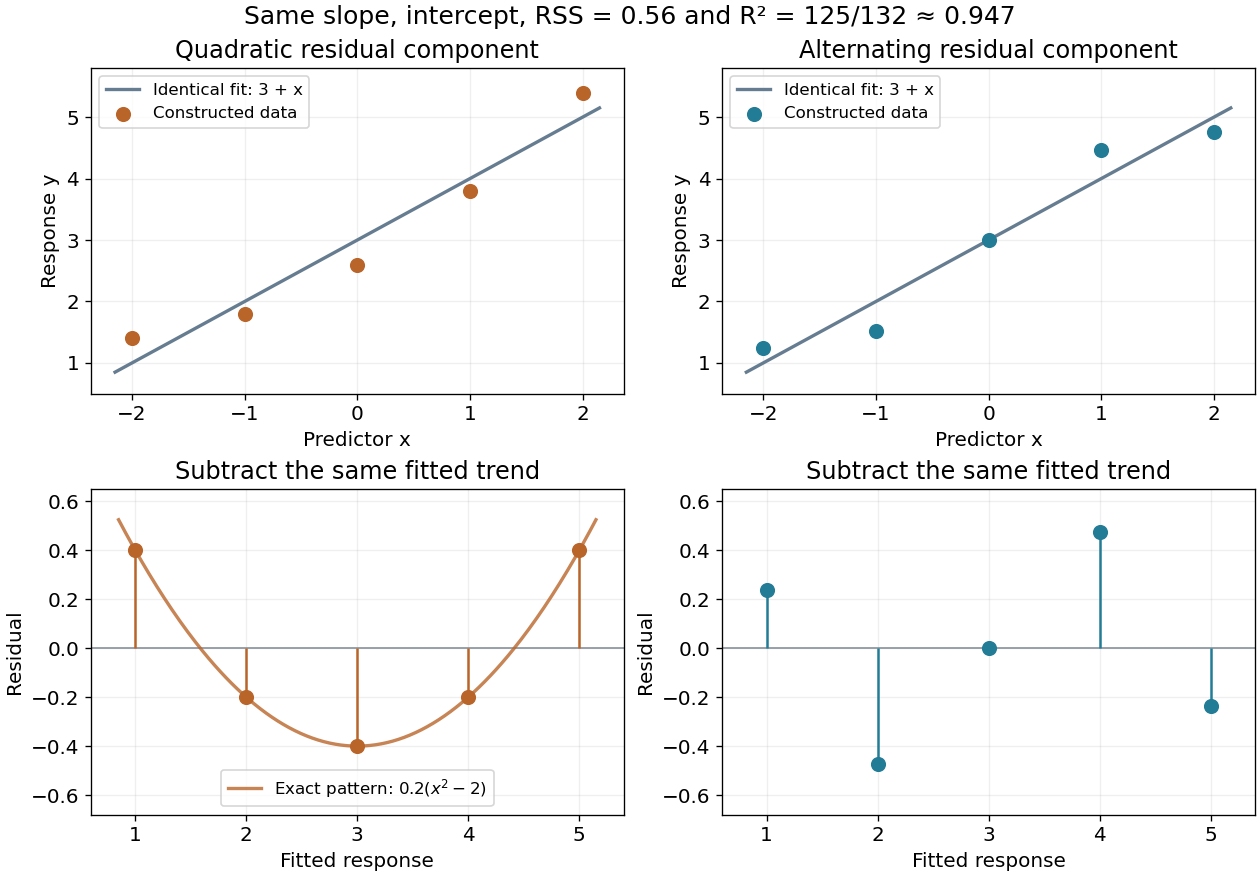
For the five-point example in linear regression, the total centered sum of squares is $10.8$ and the residual sum of squares is $0.8$, so $R^2=25/27\approx 0.926$. This summarizes the fitted reduction in squared error. It does not record the order or shape of the regression residuals, which are worth examining in a residual-versus-fitted plot.

Here is a fully constructed illustration. Use $x=(-2,-1,0,1,2)$ and the same fitted line $3+x$ for both datasets. Add respectively the residual vectorsBoth sum to zero, both have zero inner product with $x$, and both have squared norm $0.56$. Their ordinary least squares fit is therefore exactly the same line, with the same $R^2=10/(10+0.56)=125/132\approx 0.947$. But the first residual is $0.2(x^2-2)$, a systematic quadratic shape, while the second changes direction across the predictor values. These examples show directly which information the scalar $R^2$ discards; neither constructed pattern proves a random-error model.

For a full-rank ordinary least squares design matrix, the hat matrix $H$ and residual projection $G=I-H$ satisfy $HG=GH=0$. Hence fitted values and regression residuals are perpendicular as observed vectors. Under isotropic errors their cross-covariance matrix is zero, and under a normal linear model the two vectors are independent.

Fitted values are the predictions at the predictor values used to fit a regression model. In linear regression with an explicit regression intercept,Here $X$ is the slope design matrix, and $r$ is the regression residual vector. The fitted values estimate the regression function at the observed predictors; they need not equal the observed responses, which may also contain random errors. Prediction at a new predictor vector $x_{\ast }$ uses $\hat{\alpha }+x_{\ast }^T\hat{\beta }$ with the same centering and scaling used in fitting. A prediction interval addresses uncertainty in a new response rather than just displaying this point prediction.

For the five constructed observations in linear regression, ordinary least squares gives fitted values $(4/5,9/5,14/5,19/5,24/5)$. The ridge regression fit at $\lambda =10$ instead gives $(9/5,23/10,14/5,33/10,19/5)$. Both fitted vectors have sample mean $14/5$ because the regression intercept is unpenalized; their regression residuals differ and their residual sums of squares are $4/5$ and $33/10$, respectively.

For ordinary least squares, the fitted values are the orthogonal projection of $Y$ onto the column space of the complete design matrix, including its regression intercept column. They remain unique even in rank-deficient ordinary least squares, although the regression coefficients can be nonunique. The regression residuals are then orthogonal to every column.^[ref] With centered slopes, ridge regression instead satisfies $X_c^{T}r=\lambda {\hat{\beta }}_{\lambda }$, so the regression residuals need not be orthogonal to the slope columns. Their sum is still zero because the regression intercept remains free.

For fixed predictors and scales and a fixed positive penalty, ridge regression gives a linear smoother,For $\lambda >0$ with at least one nonzero slope direction, this matrix is not an orthogonal projection matrix: applying it twice shrinks that direction again. Its effective degrees of freedom are $1+{\sum }_{j=1}^r{d}_j^2/(d_j^2+\lambda )$, where $d_j$ are the positive singular values of $X_c$; the extra $1$ counts the free regression intercept. If the penalty is selected using $Y$, the resulting fitting rule need not be a linear smoother, since its chosen $H_{\lambda }$ also depends on $Y$.

With a full-column-rank $n\times p$ design and isotropic normal errors, ordinary least squares gives $\hat{\beta }\sim N_p(\beta ,{\sigma }^2(X^{T}X{)}^{-1})$, independent of the residual squared length. Orthogonal design and residual projections of the multivariate normal distribution are independent, and $\mathrm{RSS}/{\sigma }^2\sim {\chi }_{n-p}^2$. The maximum likelihood variance estimate is $\mathrm{RSS}/n$, not the unbiased estimate $\mathrm{RSS}/(n-p)$.

Linear regression models a response's conditional expectation as a linear combination of specified predictors. In matrix form,where the design matrix $X$ describes the observations, $\beta$ contains the regression coefficients, and $\epsilon$ contains the errors. The fitted values $X\hat{\beta }$ estimate the response means. The model is linear in its regression coefficients; its columns may include powers, interactions, or other transformed predictors, so polynomial regression can fit curved relationships using the same machinery.

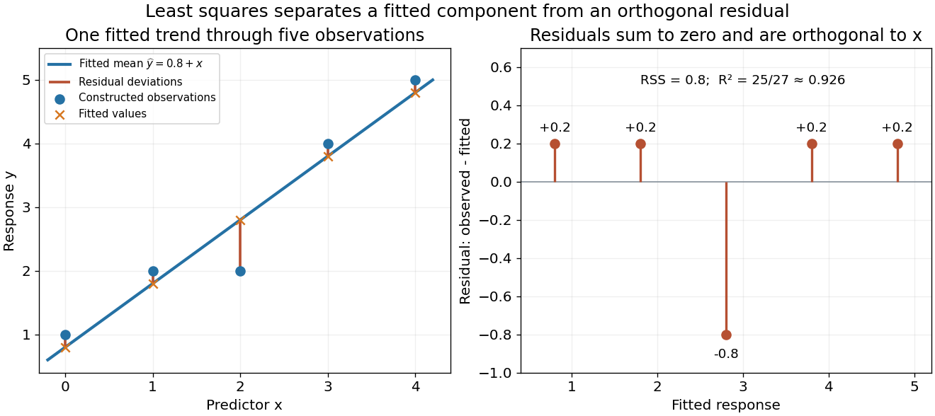
For a concrete example, take five constructed observationsAn ordinary least squares fit with an intercept gives the line $\hat{y}=0.8+x$. Its regression residuals are $(0.2,0.2,-0.8,0.2,0.2)$ and its residual sum of squares is $0.8$. A one-unit increase in the predictor corresponds to a one-unit increase in the fitted response. This is a description of this fitted association; interpreting a change as a causal effect requires the assumptions of a causal inference problem.

The geometric reason for the fit is simple. The possible mean vectors $X\beta$ form the column space of $X$. Ordinary least squares chooses the orthogonal projection of the data vector onto that vector subspace, so the remaining regression residual is orthogonal to every permitted fitted direction. The least-squares normal equations express this orthogonality as $X^T(Y-X\hat{\beta })=0$. The data's explained component and unexplained component are therefore separated by the same geometry used in a Hilbert space.

The optimization definition makes sense for any observed data. Quantifying the uncertainty of the regression coefficients needs additional assumptions about the sampling and errors. With fixed $X$ of full column rank and mean-zero errors with covariance matrix ${\sigma }^{2}I$, ordinary least squares is unbiased and has covariance ${\sigma }^2(X^{T}X{)}^{-1}$; the Gauss-Markov theorem compares it with other linear unbiased estimators. A normal linear model additionally makes Student t-distribution intervals and tests exact in finite samples. Model adequacy and predictive assessment remain relevant even when these calculations are available.

Two historical settings help explain the subject's appeal. Adrien-Marie Legendre's Nouvelles méthodes pour la détermination des orbites des comètes (1805) includes an appendix on the method of least squares: observations give more equations than unknowns, and squared errors provide a criterion for reconciling them. Its astronomical setting shows the motivation for combining imperfect measurements. ^[ref] Francis Galton's Regression Towards Mediocrity in Hereditary Stature (1886) examines the association between parental and offspring heights and the tendency of group averages toward the population average. This is a historical use of the regression name; the modern linear model is a general statistical formulation. ^[ref]

Maximum likelihood estimation is a method of statistical estimation: within a specified statistical model, choose the statistical parameter values that maximize the likelihood function of the observed data. For a parameter set $\Theta$ and observations $x$, its exact requirement isThe equality requires an attained, finite maximum; a supremum approached only at an excluded boundary is not enough. The resulting rule is a maximum-likelihood estimator. The likelihood function uses a probability mass function for discrete data and a probability density function for continuous data. See MIT 18.05, Reading 10b, sections 3 and 3.2.

The direction of the comparison is the interesting part: hold the observations fixed and vary the statistical parameter. Ten independent Bernoulli trials with eight successes and two failures give the maximum-likelihood estimate $\hat{p}=0.8$, as derived in log-likelihood. This chooses the member of the statistical model that assigns the greatest mass to that outcome. It does not assert an $80\%$ posterior probability that this parameter value is true. Bayesian statistics combines the same likelihood function with a prior distribution to obtain a posterior distribution; maximum a posteriori estimation maximizes that posterior mass or density instead.

The method turns many fitting tasks into one maximization problem. In the normal distribution model with known variance, it recovers the sample mean and ordinary least squares, while binomial regression and Poisson regression use different sampling assumptions to build their own likelihood functions. The log-likelihood turns independent contributions into a sum, exposing score equations and observed information. A peak's location gives an estimate; its shape records how much the observed data distinguish nearby parameter values.

Existence, uniqueness, bias, and statistical consistency are separate questions. Normal mean and variance maximum-likelihood estimators include a variance estimate with bias, likelihood supremum at an excluded boundary gives nonexistence, and the Neyman-Scott incidental parameter problem gives inconsistency. The usual asymptotic normality of a maximum likelihood estimator requires assumptions: a consistent estimator at an interior true parameter in a fixed finite-dimensional model with identifiability, sufficient smoothness and control of log-likelihood derivatives, and finite nonsingular Fisher information. A common parameter-independent support of a probability distribution is part of a standard sufficient framework; see Rigollet, MIT 18.650, Maximum Likelihood Estimation, slides 22-23. This is a description of the regular setting, not a complete theorem's hypotheses. The exact endpoint limit for a shifted exponential distribution shows why changing support can produce a different rate and a nonnormal limit. These properties do not follow just from maximizing a function.

In his 1922 paper in the Royal Society's Philosophical Transactions A, R. A. Fisher explicitly distinguished likelihood from probability and described choosing the parameter values with greatest likelihood. Section 6 also discusses comparing likelihoods after giving the maximum value one, the convention used in the figures here. See Fisher, On the Mathematical Foundations of Theoretical Statistics, section 6, pp. 326-328, DOI 10.1098/rsta.1922.0009.

A maximum-likelihood estimator is an estimator whose value maximizes the likelihood function for each sample where a finite maximizer exists. Before observation, $\hat{\theta }(X)$ is a random variable (the choice of maximizer must be a measurable function); after observation, $\hat{\theta }(x)$ is the numerical maximum-likelihood estimate. A formula must specify the allowed parameter set, including whether its endpoints belong to it.

For ten independent Bernoulli trials, write $K={\sum }_{i=1}^{10}{X}_i$. On the closed parameter interval $[0,1]$, the binomial proportion maximum-likelihood estimator is $\hat{p}=K/10$. Eight successes give the estimate $0.8$. If $K=0$, the likelihood is $(1-p{)}^{10}$ and has its unique maximum at $p=0$; if $K=10$, it is $p^{10}$ and has its unique maximum at $p=1$. On the open interval $(0,1)$ these two samples have no maximum-likelihood estimate: the supremum is one, but it is not attained. This is the same issue as likelihood supremum at an excluded boundary.

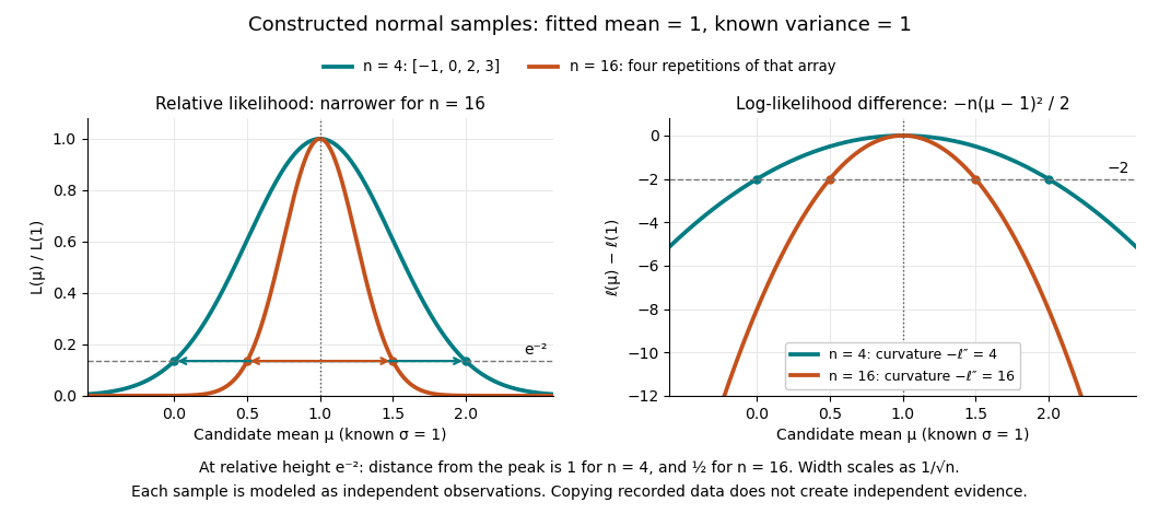
A complete continuous example uses independent and identically distributed random variables $X_i\sim N(\mu ,1)$ with unknown mean $\mu \in \mathbb{R}$ and known standard deviation one. Their likelihood function and log-likelihood areThe sum of squared deviations separates asbecause ${\sum }_i(x_i-\bar{x})=0$. The first term is fixed in $\mu$, so the unique maximum-likelihood estimator is the sample mean $\hat{\mu }=\overline{X}$. This also proves the equivalence with ordinary least squares for this model. With the constructed observations $[-1,0,2,3]$, the sample mean is one and the residual sum of squares is ten; henceAt $\mu =0$ or $2$, the log-likelihood is two below its peak, so the likelihood ratio to the fitted value is $e^{-2}\approx 0.135335$. The absolute likelihood at the peak is $(2\pi {)}^{-2}{e}^{-5}\approx 0.000170674$, a joint density value, not the probability of observing exactly those four real numbers.

The following figure compares that sample with a constructed sixteen-observation sample consisting of four repetitions of the displayed four values, modeled as sixteen independent draws. Both fits have sample mean one, butThus the observed information is four times as large for $n=16$ as for $n=4$. The distance from the peak at relative height $e^{-2}$ decreases from one to $1/2$: the width scales as $1/\sqrt{n}$. This is a comparison of two stipulated samples; merely copying recorded observations would not create new independent evidence.

Even uniqueness needs checking. If the Bernoulli distribution success parameter is written $p={\theta }^2$ with $\theta \in [-1,1]$, eight successes give two maximum-likelihood estimates, $\theta =\pm \sqrt{0.8}$, because both give the same probability distribution. The problem is a failure of identifiability. The special cases below show other ways an MLE can have bias or fail the usual asymptotic normality.

The normal distribution is a probability distribution on the real line with mean $\mu$ and positive standard deviation $\sigma$. Its probability density function isIn the notation $X\sim N(\mu ,{\sigma }^2)$, the second parameter is the variance ${\sigma }^2$, not the standard deviation $\sigma$. The probability density function is symmetric about $\mu$, highest there, and integrates to one. These formulas and the parameter convention are given in MIT 18.05, Reading 5c, §5: normal distributions.

The normal distribution is a location-scale family: if $Z$ is a standard normal random variable, then $X=\mu +\sigma Z$. Changing $\mu$ moves the center; changing $\sigma$ stretches the horizontal distances from it. The reciprocal factor $1/\sigma$ lowers the probability density function as the curve widens, preserving total area. This is why one standard normal distribution suffices to calculate probabilities for the whole family. ^[ref].

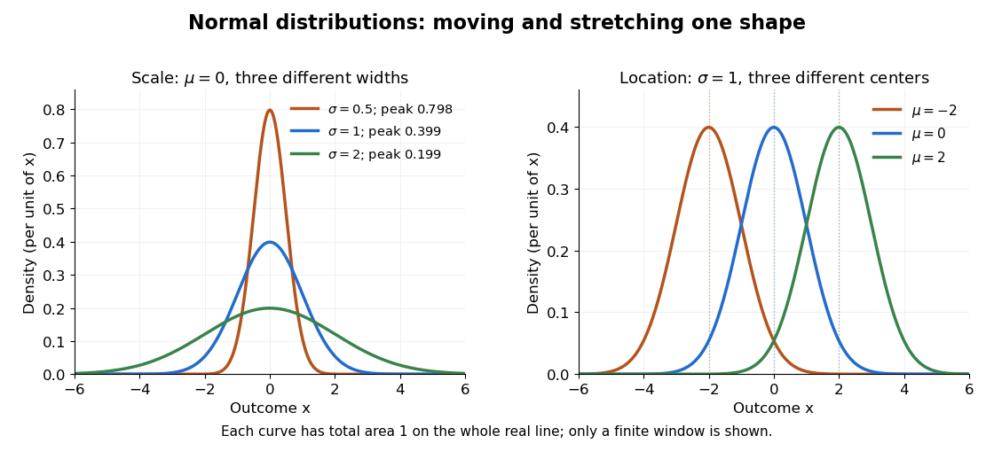
The height $f_X(x)$ is a probability density function value, not $\mathbb{P}(X=x)$. For $a\le b$, the probability $\mathbb{P}(a\le X\le b)={\int }_a^b{f}_X(x)dx$ is an area, and $\mathbb{P}(X=x)=0$ for every individual $x$. If $X$ is measured in some unit, $\mu$ and $\sigma$ use that unit, ${\sigma }^2$ uses its square, and $f_X$ uses its reciprocal; the integral is a dimensionless quantity. A change of measurement unit therefore changes the height without changing the probability. The area interpretation is developed in MIT 18.05, Reading 5b: continuous random variables.

The usefulness of the normal distribution goes beyond its simple shape. Under the central limit theorem, sums of independent and identically distributed random variables with finite positive variance, after centering and scaling, approach the standard normal distribution. Thus approximations by a normal distribution can arise even when the individual random variables have quite different probability distributions. The hypotheses matter: a model of measurement error still needs evidence that this approximation is appropriate. ^[ref]. Exact closure under a linear combination of independent normal random variables provides another reason the family is convenient.

Historically, the curve appeared in a different problem from fitting measurements. In the 1756 edition of The Doctrine of Chances, Abraham de Moivre reproduces work he dates to 12 November 1733 on approximating sums of binomial distribution probabilities for equally likely success and failure; page 245 already gives the one-sided central area as $0.341344$. ^[ref]. In his 1809 Theoria motus, Carl Friedrich Gauss derived a normal distribution for measurement error from a condition on the arithmetic mean, then connected maximizing its likelihood to minimizing the sum of squared errors under that model, the principle behind ordinary least squares. These are distinct contributions: approximating binomial distribution probabilities and justifying an estimation rule. ^[ref].

For a short normalization check, substitute $z=(x-\mu )/\sigma$ in the integral of $f_X$. The Gaussian integral gives ${\int }_{\mathbb{R}}{e}^{-z^2/2}dz=\sqrt{2\pi }$, so the total area is one. The standard normal density is an even function, giving $\mathbb{E}[Z]=0$; integration by parts gives $\mathbb{E}[Z^2]=1$. Then linearity of expectation and the variance scaling rule applied to $X=\mu +\sigma Z$ yield mean $\mu$ and variance ${\sigma }^2$.

For a linear regression design matrix $X$ with full column rank, the ordinary least squares coefficient vector is $\hat{\beta }=(X^{T}X{)}^{-1}{X}^{T}Y$. In a normal linear model with error covariance matrix ${\sigma }^{2}I$, it is an unbiased estimator with covariance matrix ${\sigma }^2(X^{T}X{)}^{-1}$. Replacing ${\sigma }^2$ by the residual variance estimate gives the reported coefficient standard errors.

In simple linear regression with a nonconstant predictor,

Partial regression first projects a response and a selected predictor orthogonally off the remaining design columns. Regressing the residualized response on the residualized predictor yields its coefficient in the full ordinary least squares fit.

For the general normal linear model, minimizing $\Vert Y-X\beta {\Vert }^2$ gives the least-squares normal equations $X^{T}X\hat{\beta }=X^{T}Y$. Full column rank makes $X^{T}X$ invertible, soThe mean and covariance follow by substituting $Y=X\beta +ϵ$ and using $\mathbb{E}ϵ=0$, $\mathrm{Cov}(ϵ)={\sigma }^{2}I$. Normal errors also give the exact multivariate normal distribution of this estimator.

Use coded experimental variablesTheir origin is the middle of the allowed rectangle, and the stated endpoints become $\pm 1$. The four corners and $n_0$ center runs give mutually orthogonal columns $1,x_1,x_2$, withWriting ${\bar{Y}}_0=n_0^{-1}{\sum }_{i=5}^{4+n_0}{Y}_i$ when $n_0>0$, the ordinary least squares estimates areTheir variances are ${\sigma }^2/(4+n_0)$, ${\sigma }^2/4$, ${\sigma }^2/4$, with zero covariances.

The repeated center runs estimate pure error without requiring the fitted mean surface to be correct:They also permit a center-point curvature contrast. Let ${\bar{Y}}_F=(Y_1+Y_2+Y_3+Y_4)/4$ and $\hat{\gamma }={\bar{Y}}_F-{\bar{Y}}_0$. Under the first-order model, $\mathbb{E}\hat{\gamma }=0$ and $\mathrm{Var}(\hat{\gamma })={\sigma }^2(1/4+1/n_0)$. Under a quadratic surface, its expectation is ${\beta }_{11}+{\beta }_{22}$, since the linear and $x_1{x}_2$ terms average to zero. Thusunder the first-order normal model. With only one center run there is no pure-error degree of freedom. A zero center contrast does not exclude all curvature, because the two quadratic coefficients can cancel. The corners also estimate an interaction contrast; the full Lack-of-fit F-test compares the first-order fit with the five setting means, with two lack-of-fit and $n_0-1$ pure-error degrees of freedom.

If the first-order model is adequate and $\hat{b}=({\hat{\beta }}_1,{\hat{\beta }}_2{)}^T\ne 0$, steepest ascent in response surface methodology uses the unit coded direction $d=\hat{b}/\Vert \hat{b}\Vert$. The Cauchy-Schwarz inequality proves that it maximizes the predicted directional derivative. Run sequential settings $x=hd$ for increasing feasible $h$, corresponding to physical increments $(5h{d}_1,2.5h{d}_2)$ from the center. Stop or reduce the steps when measured yield ceases to improve, and refit locally near promising settings. Respect the allowed rectangle; if a boundary is reached, investigate feasible boundary directions rather than extrapolating outside it. A near-zero gradient offers no first-order ascent direction and calls for further modeling.

If curvature is indicated, add the four axial settings $(1,0),(-1,0),(0,1),(0,-1)$, together with further center replication. This face-centered central composite design stays inside the allowed physical ranges and separates the two squared coordinates, which the corners alone cannot do. Fit the full quadratic regression surfaceWrite its fitted quadratic part as $x^{T}Bx$, where $B_{11}={\hat{\beta }}_{11}$, $B_{22}={\hat{\beta }}_{22}$ and $B_{12}=B_{21}={\hat{\beta }}_{12}/2$. Its gradient and Hessian are $\hat{b}+2Bx$ and $2B$. If $B$ is nonsingular, the stationary setting isIf $B$ is negative definite and $x_{\ast }$ is feasible, it is the fitted maximum. Otherwise compare feasible stationary settings, optima on each edge obtained from the restricted one-variable quadratic, and the corners. A singular or poorly determined $B$ calls for attention to ridge directions and more runs. Convert any chosen coded setting back using ${\xi }_1=95+5x_1$, ${\xi }_2=37.5+2.5x_2$, and confirm its yield experimentally. The fitted local surface guides the search; it does not establish an untested physical optimum.

Put $z_i=x_i-\bar{x}$, so $\sum z_i=0$. The ordinary least squares criterion is $S(\alpha ,\beta )={\sum }_i(Y_i-\alpha -\beta z_i{)}^2$. Setting both partial derivatives to zero gives ${\sum }_i(Y_i-\alpha -\beta z_i)=0$ and ${\sum }_i{z}_i(Y_i-\alpha -\beta z_i)=0$. Therefore, provided $S_{xx}=\sum z_i^2>0$, the centred simple linear regression estimators areThe Hessian of $S$ is $2\mathrm{diag}(n,S_{xx})$, which is positive definite, so this stationary point is the unique minimum. From the mean-zero errors, both estimators are unbiased; independence and common error variance give $\mathrm{Var}\hat{\alpha }={\sigma }^2/n$, $\mathrm{Var}\hat{\beta }={\sigma }^2/S_{xx}$, and zero covariance. Normality is not needed for this derivation. If all $x_i$ coincide, the slope is not identifiable and only the intercept is determined.

Using the PDF data gives $\bar{x}=6.2$, $\bar{y}=42.4$, $S_{xx}=86.8$ and $S_{xy}=-257.4$. In particular, the fourth cost is 37 in the PDF; the TeX's 75 is a transcription error and would contradict the supplied covariance sum. The fitted simple linear regression isHere the centred intercept estimate is 42.4; an intercept at $x=0$ would instead be $\hat{\alpha }-\hat{\beta }\bar{x}$. For eight units the predicted unit cost is

The commands read the 52 cell values into a vector and build the matching two-factor layout. In expand.grid(country, goods) the first factor varies fastest, so the four countries are listed successively within each goods category. This matches row-by-row reading of the displayed table. Converting Goods to a factor is essential: its labels identify 13 categories and are not a quantitative trend. Country supplies the other categorical factor. The summaries suppress coefficient correlations, not coefficient standard errors.

The first fit is the additive two-factor normal linear modelThere are $1+12+3=16$ free coefficients and $52-16=36$ residual statistical degrees of freedom. This is two-way analysis of variance without an interaction term. For this complete balanced layout, ordinary least squares givesThese formulas follow from the row- and column-sum normal equations: fitted row and column totals equal their observed totals. The balanced-design coefficient standard errors are $s\sqrt{2/4}$ for a goods contrast, $s\sqrt{2/13}$ for a country contrast, and $s\sqrt{1/4+1/13-1/52}$ for the reference-cell intercept. These yield the common contrast standard errors and the different intercept standard error in each summary. In particular the intercept is the fitted Software–UK value, not the grand mean or the observed Software–UK entry.

Thus the first intercept predicts $149.8269$ million euros for Software in the UK. The Books coefficient adds $254.7$ million euros to the fitted value in any country, relative to Software; every other goods coefficient has this same arithmetic-difference interpretation. The country coefficients subtract $193.7$, $57.0308$ and $97.3769$ million euros from the UK prediction for France, Germany and the rest of Europe respectively, regardless of goods. The model therefore assumes common absolute country differences across goods categories. For Software–France its prediction iswhich is impossible for positive spending and indicates a limitation of this additive original-scale specification.

The residual standard error is $80.98$ million euros, obtained from $s^2=\mathrm{RSS}/36$; direct calculation gives $\mathrm{RSS}=236088.7435$. Each coefficient's printed statistic is $\hat{\theta }/\mathrm{se}(\hat{\theta })$, with a $t_{36}$ reference distribution under this normal linear model. The two-sided p-values compare each goods category with Software, or each other country with the UK, after adjustment for the other factor. For example France and the rest of Europe differ significantly from the UK at 5%, but Germany does not. The raw-scale significant goods differences are Books, Clothing, Electronic Goods, Groceries and Leisure Travel; these are individual reference-level comparisons, not an overall test of the goods factor.

The coefficient of determination is $R^2=1-\mathrm{RSS}/\mathrm{TSS}=0.7743$. The omnibus F-test compares all 15 nonintercept coefficients with zero:with reference $F_{15,36}$ and $p=1.2544\times 10^{-7}$. This says at least one factor contrast is nonzero under the assumed error model. There is one observation per cell, so an unrestricted goods-country interaction would saturate the model, leaving zero residual degrees of freedom. Without replication or a specified interaction structure, the residual variation cannot be separated into interaction and independent error.

The second fit applies a logarithmic transformation and fits the same factor design to $Z_{gc}=\log Y_{gc}$. The Gaussian log-response model isIts intercept exponentiates to a fitted Software–UK conditional median of $e^{4.5267}\approx 92.45$ million euros. Goods coefficients now give multiplicative ratios to Software, and country coefficients give multiplicative ratios to the UK. The estimated country ratios areFor example the Books ratio is $e^{1.6415}\approx 5.16$ and the Sports Equipment ratio is $e^{-1.8364}\approx 0.1594$, consistently across countries. The model assumes common relative, rather than common absolute, country effects. It also guarantees positive retransformed fitted values. Under normal log errors, the original-scale conditional mean is $e^{\eta +{\sigma }^2/2}$, whereas $e^{\eta }$ is the conditional median and geometric mean. Correcting the retransformation bias here multiplies the naive predictions by approximately $e^{0.127406/2}=1.0658$.

The log-scale residual standard error is $0.3569$, with the same 36 residual degrees of freedom, corresponding to a typical multiplicative error multiplier $e^{0.3569}\approx 1.429$. France and the rest remain significant reference-country contrasts; Germany remains nonsignificant at 5%. The log-scale significant reference-goods contrasts are Books, Music, Videos/DVDs, Clothing, Sports Equipment, Electronic Goods, Groceries and Leisure Travel. Event Tickets, Toys, Video Games and Housewares do not individually differ significantly from Software at that level. These p-values remain subject to the usual multiple testing qualification.

The log-scale $R^2=0.9381$ is computed using variation in the logarithms, so it cannot by itself establish better fit on the original response scale. The change is plausible because spending varies widely in magnitude and relative discrepancies are more meaningful than constant absolute discrepancies, but it should be assessed with regression diagnostics, especially a residual-versus-fitted plot and a normal Q-Q plot. The minimum residual near $-1.01$ merits inspection; the command summaries alone do not verify independent normal errors. Moreover these responses are forecasts, so the inferential p-values have a literal sampling interpretation only if an appropriate stochastic model for their uncertainty is justified.

The log-scale analysis of variance adds Goods and then Country. In this balanced design their effect spaces are orthogonal after removing the intercept, so the sequential sums of squares equal the corresponding adjusted factor sums and are unchanged by reversing the two factors:The residual sum of squares is $4.58662$, giving $M{S}_E=4.58662/36=0.127406$. ThusTheir tiny upper-tail p-values show strong overall goods and country effects under the log-error model; a globally significant country factor is compatible with the nonsignificant individual Germany contrast. The omnibus fit statistic is $36.3433$ on $(15,36)$ degrees of freedom, whose p-value is approximately $3.14\times 10^{-17}$. The printed zero reflects numerical formatting, not an exactly zero probability.

If two cell entries were missing, retain their correct factor labels and mark those responses unavailable, rather than shifting the remaining scan values into different cells. Fit the additive models to the 50 observed cells, assuming the missingness mechanism permits those observations to be analyzed without selection bias. All factor levels remain represented, and the row-column incidence graph remains connected: any two goods rows still share an observed country, since only two edges of the complete layout have been removed, and every country still has many observed goods. By identifiability of an incomplete two-factor additive design, the design therefore still has rank $13+4-1=16$. HenceThe coefficients and their covariance must be recomputed by the observed-cell ordinary least squares equations. The balanced row-mean-plus-column-mean formulas and common within-factor standard errors no longer apply. Goods and Country effects are generally no longer orthogonal, so sequential ANOVA sums can depend on order; factor tests adjusted for the other factor should use nested model comparisons. Missing cells do not restore replication or make an unrestricted interaction test possible: that larger model still fits every observed cell exactly. If missingness depends on the unavailable spending values, additional modelling of that mechanism would be needed.

Expanding the ordinary least squares objective givesFor a nonzero vector $v$, $v^T{X}^{T}Xv=\Vert Xv{\Vert }^2>0$, since the design matrix has matrix rank $p$. The Hessian matrix is therefore positive-definite, and $Q$ is strictly convex. Solving its normal equations gives the unique least-squares estimator:Indeed, expansion about this stationary point and $X^T(Y-X\hat{\beta })=0$ give $Q(\beta )=Q(\hat{\beta })+(\beta -\hat{\beta }{)}^T{X}^{T}X(\beta -\hat{\beta })$, which also proves the global minimum directly.

Define the hat matrix $H=X(X^{T}X{)}^{-1}{X}^T$. It is a symmetric matrix and an idempotent linear map, since $H^T=H$ and $H^2=H$, and its image is the column space of $X$. Thus $H$ is the orthogonal projection onto the fitted mean space. The fitted values are $HY$ and the regression residual vector is $(I-H)Y$. Because $I-H$ is also a symmetric matrix and an idempotent linear map,These minimization and projection identities do not need errors with a normal distribution; the normal linear model becomes relevant to the distributional calculations.

The plug-in estimate isFor a concrete bootstrap construction, suppose the rows $(x_i,y_i)$ are independent and identically distributed, $\mathbb{E}(e_i\mid x_i)=0$, the design moment matrix is nonsingular, and the required moments exist. Use a paired bootstrap: sample $n$ rows with replacement, form $X^{\ast },Y^{\ast }$, refit by ordinary least squares, and compute ${\hat{\theta }}^{\ast }={\hat{\beta }}_1^{\ast }{\hat{\beta }}_2^{\ast }$. Repeat many times. Singular resampled designs require a suitable rank-preserving implementation or replacement replicate; with a regular continuous design their frequency vanishes asymptotically.

The bootstrap-t confidence interval method also needs a standard error in the original sample and every replicate. One asymptotically valid heteroscedasticity-robust covariance estimate isThe delta method for the coefficient product givesRecompute ${\hat{V}}^{\ast },d^{\ast },{\hat{s}}^{\ast }$ in each paired replicate. This is bootstrap inference for a product of regression coefficients.

With fixed rather than random design, resample centered residuals if errors are identically distributed with homoskedasticity, or use a properly specified wild bootstrap for heteroscedastic errors, keeping $X$ fixed and refitting after generating $Y^{\ast }$. The printed assumption $\mathbb{E}{e}_i=0$ alone does not establish independent observations or validity of a bootstrap confidence interval. The formulas below give asymptotic 95% coverage under the stated regularity conditions, not an exact finite-sample guarantee. In particular the ordinary first-order studentization needs $({\beta }_1,{\beta }_2)\ne (0,0)$ and a nonzero asymptotic variance; when both coefficients vanish the product has nonstandard behavior.