The source bundle filename differs from the examination year; the cover identifies Trinity Term 2021. The solutions below retain the printed conventions where consistent and explain the corrections needed elsewhere.
The printed magnetic dipole moment uses dimensionless angular momentum operators: their physical counterparts are and . Choose the magnetic field along . Then the Zeeman energy is , whose characteristic size is . In LS coupling, treating this as a time-independent perturbation theory requires it to be much smaller than the relevant fine structure separation, rather than merely smaller than the Coulomb interaction energy.
For a concrete hydrogen atom estimate take the pair. The hydrogen fine-structure correction iswhere is the fine-structure constant, distinguished from the later potential coefficient. ThusConsequently a suitable weak-magnetic field condition for this pair isThere is no single threshold for every hydrogen energy level: the relevant fine structure separations decrease with . The energy level has no same- spin-orbit interaction partner, so it cannot itself define this comparison. This calculation neglects hyperfine structure; resolving that smaller scale requires an additional weak-magnetic field condition.
Within a fixed angular momentum multiplet, the component of along follows from . The corresponding result for follows by interchanging and . For the quantum state ,These are dimensionless expectation values in the convention of part (a). Substituting into the first-order time-independent perturbation theory formula givesFor , the Landé g-factor becomesThe magnetic sublevels must first be diagonalized within a degenerate multiplet; choosing along the magnetic field already does this. For the displayed fraction is undefined, but all vector expectation values vanish and there is no first-order Zeeman splitting. A higher-order shift may remain.
Write and retain the nuclear Coulomb potential. In spherical coordinates, the total potential energy iswhen ; is a Legendre polynomial. Treat the added term using quadratic anisotropic perturbation of hydrogen and degenerate perturbation theory in the hydrogen energy eigenbasis. It preserves parity and , so it cannot mix with , or distinct magnetic sublevels.
For a hydrogen atom, the hydrogen radial second moment givesThe angular expectation values of are for an orbital, for , and for , obtained by integrating the squared spherical harmonics. Therefore the five lowest spatial quantum states, counting statistical weight, have first-order energy levelsEach spatial quantum state has two electron spin states when spin-orbit coupling and the magnetic field are omitted. Thus these are five spatial states but only three distinct first-order energies; five distinct energies would be an incorrect reading. The accidental equality can be lifted at higher order. Quantitatively the added shifts must also be small compared with neighboring principal-shell gaps; is an asymptotic condition, not a guarantee for arbitrary large .
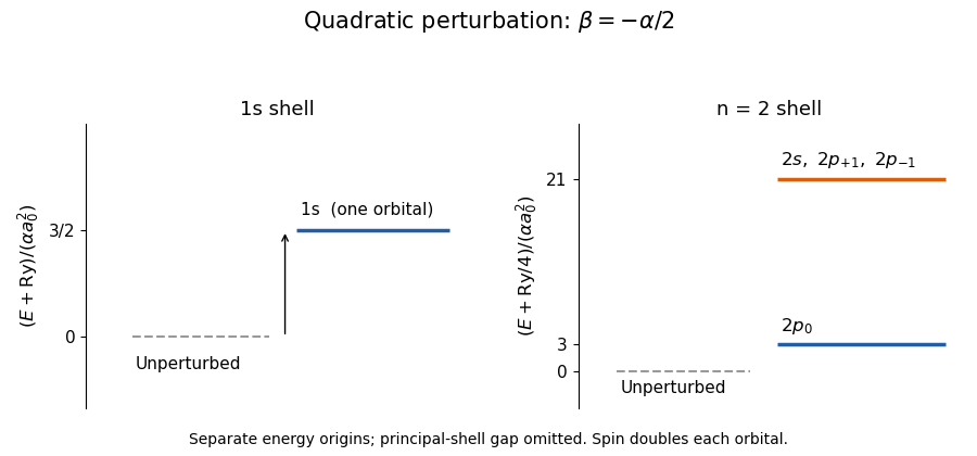
First-order spatial levels of locally perturbed hydrogen; the gap between principal shells is compressed
. Details. For general , the expectation value isIt does not cancel every order. At , couples to orbitals. For example its angular matrix element with is , and the radial matrix element is nonzero. The second-order nondegenerate perturbation theory sum has negative denominators, so this is a concrete nonzero higher-order contribution.
There is also a global limitation: for either negative above, . A localized wavepacket translated far along has fixed kinetic energy but arbitrarily negative potential energy, proving there is no true lowest energy level. The results describe local perturbative resonance poles, or a potential completed to a confining form far from the atomic nucleus. No globally exact ground-state cancellation exists for the potential as printed.
Neglect hyperfine structure, spin-orbit coupling and the diamagnetic term, and set , . The Zeeman energy is . The electron spin is free, so every spatial result below is duplicated with an added .
For a magnetic field parallel to , the old magnetic quantum number remains good and the first-order energy levels areThe two orbitals have zero orbital angular momentum, so only their electron spin contributes at this order.
For a magnetic field parallel to , the expectation of in each individual orbital vanishes. One must still check the degenerate subspace: its projected is zero as well. Thus there is no first-order orbital splitting in a sufficiently weak transverse magnetic field. Spin still contributes .
The transverse orbital Zeeman mixing can be seen without assuming its size. Put , , and . In the real orbital basis, is unaffected while have off-diagonal matrix elements of modulus . Diagonalizing this two-dimensional Hamiltonian gives the spatial energy eigenvaluesWhen , their shifts relative to the earlier levels are , with added for electron spin. The displayed square-root expression also handles comparable to , provided coupling to other principal shells stays negligible. The orbital retains zero orbital correction.
These quadratic orbital estimates keep the enhanced contribution from mixing the split levels. Minimal magnetic minimal coupling also produces ; its expectation value is positive and must be added for a full order- calculation. For example it gives for . It is parametrically smaller than the mixing term when .
Expand the wavefunction in unperturbed energy eigenstates,The are interaction picture probability amplitudes, so are level populations and in this closed two-level system. A classical field supplies the electric-dipole interaction . Choosing the relative phase of the energy eigenstates makes real. This is the resonant Rabi angular frequency.
Combining the field's two exponentials with the unperturbed quantum phases produces terms oscillating at and at . The rotating-wave approximation drops the latter, leaving exactly the supplied equations with coupling . It requires and a field envelope slow enough on the carrier timescale. Spontaneous emission and dephasing must be negligible during the sequence. For a ground-state hyperfine level transition, the analogous direct drive is a magnetic dipole transition; the same equations hold with the magnetic matrix element replacing the electric one.
Assume an initially unexcited chemical atom, two nonoverlapping square pulses starting at , and a common coherent field phase. In the weak-excitation limit , substitute into the second probability amplitude equation. After the second pulse,where the sinc function means , with value one at zero. Squaring givesThe printed prefactor is a factor of four too small for the supplied equations and pulse durations. A direct counterexample is : the exact resonant Rabi oscillation gives for two pulses of duration , because the intervening resonant rotating-frame evolution is trivial. Its small-area limit is , rather than . The latter is the single-pulse result before coherent addition.
The condition printed in the source also does not justify the derivation from a physical carrier field. A consistent rotating-wave approximation pulse regime isIf the supplied equations are treated as the mathematical model regardless, their weak-excitation integral remains valid for any ; subcycle pulses of the original real field require the discarded counter-rotating term and depend on carrier phase. here is the separation of pulse starts, as specified, rather than the dark interval .
The ground electron configuration of caesium has a single electron, with . Addition of angular momentum giving fixes the nuclear spin to . With dimensionless angular momentum operators, write the Fermi contact interaction asThe two hyperfine levels therefore differ by . In the convention and ,This exposes a missing ingredient in a prediction from the supplied data: and alone do not specify the valence electron contact density. Screening effect and penetration of the closed core strongly affect it. If instead denotes the total nuclear moment in units of , it must first be divided by in the displayed convention.
An explicitly crude unscreened hydrogen-like ion model uses and gives , or . It describes neither the shielding nor the radial function of neutral caesium. Using a pure unit-charge hydrogen orbital instead gives only , illustrating why a unique useful estimate cannot follow from an unspecified effective charge.
For physical neutral , the independently known zero-magnetic field clock transition isThis measured frequency, used to define the second, is supplementary physical information, not a consequence of and the rounded alone.[ref]
SI base unit: second (s) by Bureau International des Poids et Mesures. Definition: the unperturbed ground-state hyperfine transition frequency of caesium-133 is exactly 9 192 631 770 Hz
The direct electronic transition is in the microwave range and is a magnetic dipole transition, rather than a direct optical electric dipole transition. An optical implementation needs a two-field Raman transition.Using the corrected weak-pulse Ramsey spectrum of part (b), the peak at has height . The quantum interference fringes have spacing in angular frequency, with zeros at , and the sinc function envelope has its first zeros at . For , the central peak has approximately full width at half maximum in angular frequency. The clock transition between the two states has no first-order Zeeman energy, although a quadratic one remains.
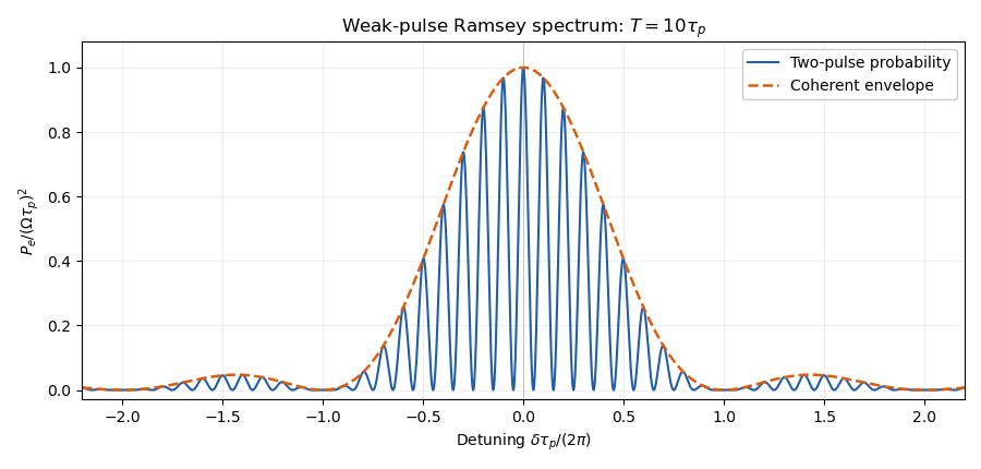


The first-order excitation amplitude is the Fourier transform of the temporal pulse envelope evaluated at the Rabi detuning. Two rectangular time windows therefore give exactly the mathematical structure of double-slit interference: each window gives a sinc function amplitude, and their separation gives a relative quantum phase . The transition probability is a sinc function squared envelope multiplied by .
Pulse duration corresponds to slit width, pulse-start separation to slit-center separation, and Rabi detuning to the transverse wavevector sampled on the screen. The narrow fringes measure the long separation, while the broad envelope measures the short interaction duration. As in spatial interference, adding probabilities instead of coherent probability amplitudes would lose the fringes. Randomizing the relative pulse phase averages the cosine squared to .
Differentiating the specified rotating-frame amplitudes gives the time-independent Schrödinger equationThe characteristic polynomial is , henceFor , corresponding normalized eigenvectors are proportional to . Their arbitrary complex coefficients evolve as ; this solves the amplitude equations for any initial quantum state.
Restoring the common energy origin , the two dressed state energy eigenvalues areThus their positive energy separation increases byEquivalently, the branches connected to and shift by and respectively. Their signed difference changes by , which is the printed expression with a signed convention. For negative Rabi detuning, an actual positive separation still increases; for example at it cannot have the negative change implied by reading the printed expression as an unsigned gap. These opposite AC Stark shifts describe level repulsion.
Specify the radiation normalization first. Let be radiation energy density per ordinary frequency, with SI units . Then is the spontaneous emission rate per upper-state chemical atom, while and are the induced absorption and stimulated emission rates, evaluated at a sharp transition frequency. For a finite spectral line profile, replace by its profile-weighted average.
The Einstein coefficients obeyHere are the statistical weights of the two energy levels, and the field is unpolarized and isotropic. The units and physical dimensions areThe apparently time-independent dimension of follows because a per-hertz density includes an extra unit of time. If instead multiplies the mean intensity , use and . These distinct normalizations must not be mixed in the radiative transfer equation.
Use the energy-density convention of part (a), a normalized common spectral line profile , and isotropic spontaneous emission. For a narrow spectral line centered at ,The factor follows from : angle-integrated absorption removes of energy per volume and time. The emission coefficient is per solid angle, whereas the absorption coefficient has units of inverse length.
The Boltzmann distribution in thermal equilibrium gives . Dividing the two expressions and using the relations between Einstein coefficients,Thus the source function equals the Planck function at the transition frequency, and in the usual narrow-line approximationWith an exactly common finite-width and constant line-center Einstein coefficients, their ratio is constant across the profile; exact equality to a varying at every frequency is only a narrow-line approximation. Exact thermal radiative transfer requires frequency-resolved detailed balance, which supplies the corresponding small profile corrections. This distinction does not alter the intended equilibrium result.
For constant nonzero absorption coefficient, multiply the radiative transfer equation by the integrating factor :Integrating from the entrance to givesThe boundary condition is immediate. Differentiation gives , checking the equation. For positive optical depth , the incident specific intensity is forgotten and . Negative absorption coefficient instead describes gain and does not have this relaxation limit. At use the nonsingular form directly: .
In local thermodynamic equilibrium, write the one-ray radiative transfer equation asLarge total optical depth removes the boundary contribution, but an additional local condition is essential: the temperature and opacity vary little over an absorption length . Iterating once in that small gradient givesThe integrated Planck function and its derivative areUsing the specified Rosseland mean opacity, with measured here in inverse length, the source's definition therefore givesThe printed leading term lacks a factor under that definition. An isothermal optically thick medium is a concrete counterexample: gives exactly, while the printed formula gives .
A physical radiative flux requires an angular integral. For direction cosine , the same gradient expansion gives . Integration over all directions gives the net radiative diffusion fluxThe isotropic equilibrium contribution cancels between opposite directions. For comparison the outward-hemisphere flux alone is at this order. None of these consistent definitions yields the printed mixture of coefficients.
To derive fermionic Einstein-coefficient relations, first consider an idealized emitter that can exchange one ultrarelativistic fermion with the bath, with zero chemical potential. Let be its density of states per volume and ordinary frequency, with populated helicity states; for one neutrino helicity , whereas the corresponding photon count is two. The Fermi-Dirac distribution givesPauli blocking changes the final-state factor in downward emission from the bosonic to . Define positive coefficients and . The upward rate per lower emitter is , and the downward rate per upper emitter isThermal detailed balance, with , yieldsFor example, substituting reduces the balance equation to because .
If one insists on the original additive notation , its formal coefficient is negative:A negative correction means inhibited emission into occupied modes, not a negative total decay rate; ensures positivity. The dimensions are those of part (a), and the factor of two relative to the photon density is a helicity count, independent of the statistical sign.
There is a physical qualification: ordinary electronic energy levels of the same chemical atom have the same fermion parity, and cannot interconvert by emission or absorption of a single neutrino. A realizable single-fermion emitter must change the relevant particle-number and parity sector, with matching conservation laws. For ordinary atomic levels, neutrino-pair processes would require a different calculation. A bath with nonzero chemical potential would also require the corresponding chemical-equilibrium population ratio. The calculation above is the intended single-mode statistical analogy under explicit assumptions.
The closed shells have , leaving the equivalent electrons. Addition of angular momentum and the Pauli exclusion principle permit the atomic terms . Their term symbols use . Hund's rules put the triplet state below the singlet states; for a less-than-half-filled shell the smallest in is lowest. ThusAll have even parity. These assignments agree with independent tabulated carbon energy levels.[ref]
Energy Levels of Neutral Carbon by National Institute of Standards and Technology. 2s²2p² entries: ³P₀,₁,₂ at 0, 16.41671 and 43.41350 cm⁻¹; ¹D₂ at 10192.66 cm⁻¹; ¹S₀ at 21648.02 cm⁻¹
The rounded source values should not be forced to satisfy an exact Landé interval rule; pure first-order LS coupling need not account for every measured fine structure correction.For two decays from a common upper energy level, their photon wavenumber difference equals the separation of the two lower energy levels. Treating both quoted wavelengths as vacuum values initially giveswhose difference is close to . The only matching lower pair among the supplied energy levels is , with the shorter-wavelength photon ending on . The two independent upper energy estimates areThusThe electric-dipole selection rules require odd parity, , and to connect to both singlet lower energy levels. The apparent discrepancy has a concrete convention explanation. The NIST carbon line table lists under vacuum wavelengths and under air wavelengths, reproducing the source's rounded numbers.[ref]
Strong Lines of Carbon by National Institute of Standards and Technology. Vacuum section: C I 1930.906 Å; air section: C I 2478.561 Å
The second number must therefore be converted to a vacuum wavelength before using . For the tabulated upper and lower energy levels, its vacuum wavelength is , corresponding to an air refractive index about . This removes the spurious discrepancy. The first calculation alone, which correctly uses a vacuum wavelength, already gives the intended upper energy level to the accuracy of the rounded data. The independent upper value is .[ref]Energy Levels of Neutral Carbon by National Institute of Standards and Technology. 2s²2p(²P°)3s ¹P°₁ entry at 61981.82 cm⁻¹
In the idealized isolated-carbon chemical atom interpretation, both beams carry approximately per incident particle, close to the threshold. However equal incident energies do not imply equal excitation channels.
A single optical photon cannot strongly excite any of the listed even-parity energy levels from the even-parity ground state through an electric dipole transition. In particular also violates and the restriction. The lowest strong opposite-parity excitations lie well above . Thus one expects no strong resonant absorption or corresponding strong atomic fluorescence from these ground-state chemical atoms at this optical wavelength; weak higher-order processes and scattering are separate effects.
Incident electrons can undergo inelastic scattering and collisional excitation. Their orbital angular momentum and exchange with bound electrons allow transfers excluded for a single electric dipole photon. The energy level at and the low fine structure excitations are energetically accessible. One therefore expects scattered electrons with discrete energy losses, possible weak forbidden spectral lines, and collisional or surface relaxation. For example has wavelength approximately ; spin mixing supplies the weak spin-forbidden radiative channel.
There is a numerical threshold caveat. Literally,Neither quoted beam reaches from the exact ground state if these are taken as exact monoenergetic values. The electron value rounded to two decimal places could represent an actual energy above threshold; if so, is collisionally accessible and its decay to produces the weak electric quadrupole transition at , followed by lower-level relaxation. These emissions require populations and sufficiently low collisional quenching of a metastable line.
An actual solid carbon foil has bands, collective excitations and surface losses, so it need not reproduce the isolated-chemical atom spectrum or selection rules. Its optical and electron-induced emission cannot be predicted quantitatively from the five atomic energy levels alone. This is the limitation of the foil wording in the source.
Take the initial ground-state chemical atom at rest in the laboratory. The incident photon has energy and momentum . The excited chemical atom has rest mass and must carry that momentum. Conservation of energy and conservation of momentum giveSquaring cancels the photon-energy square:ConsequentlyThe extra positive term is the photon absorption recoil correction and supplies atomic recoil energy. The formula is exact for the initially stationary isolated chemical atom; it does not assume . Initial and final chemical atoms cannot both remain at rest during single-photon absorption without another body taking momentum.
Put . Gauss's law for a uniform spherical nuclear charge distribution, with the electrostatic potential matched at , gives the electronic potential energySubtracting the point-nucleus Coulomb potential leaves the nonnegative perturbationThe normalized nonrelativistic hydrogen-like ion wavefunction has . Since , approximate it inside the atomic nucleus by . First-order time-independent perturbation theory then givesDefine , as the paper specifies for the hydrogen-like ion, rather than the neutral-hydrogen value. Using givesto leading order in . For , , , andThe finite nuclear charge radius makes the energy level less bound. The quoted frequency is a level shift divided by : a line frequency shifts by , so a decay into this shifted level alone has the opposite sign.
The formula is a nonrelativistic, small-nuclear charge radius estimate. Keeping the exponential in the first-order integral gives , about a one-percent correction here. More seriously, for lead, so relativistic contraction is substantial. A precise physical prediction needs a finite-nucleus Dirac equation calculation; the boxed estimate is the model requested, not precision heavy-ion spectroscopy.
A nonrelativistic wavefunction vanishes linearly at the origin. Its probability density is therefore proportional to , so its first-order finite nuclear size correction shift scales as , rather than the result for . It is positive but much smaller.
More explicitly, the normalized hydrogen-like ion radial function obeys near the origin. Since the spherical harmonic has unit angular norm,ThusThis is about in the nonrelativistic model. At large , the relativistic Dirac spinor has an -type small component and a much stronger nuclear sensitivity than this nonrelativistic argument predicts; remains much more suppressed. Neglecting spin-orbit interaction corrections would miss that distinction.
The finite nuclear size correction perturbation is unchanged for the same lead atomic nucleus. Its leading effect on one occupied orbital is still proportional to that orbital's contact density,Other electrons screen the nuclear attraction and alter the self-consistent wavefunction, usually reducing its contact density and hence its positive shift relative to the bare hydrogen-like ion. The reduction is modest for a deep orbital: it penetrates well inside most other shells and still samples nearly the full attraction. Replacing by the neutral atom's asymptotic charge one would be inappropriate for this core orbital.
A neutral lead atom has two electrons. Their contributions add in a frozen-orbital estimate of total atomic energy, roughly twice the per-electron shift, with relaxation and correlation corrections. An experimentally observed transition frequency again depends on the difference between the finite-size shifts of both participating many-electron quantum states. A quantitative neutral-lead result requires a screened relativistic many-electron calculation, not the one-electron formula with a single universally valid effective charge.
Articles by others on the same topic
There are currently no matching articles.