Use completing the square rather than computing the eigenvalues of the symmetric matrix. Successively removing the mixed terms givesThus one suitable invertible linear change of coordinates isThe coordinate matrix is upper triangular with determinant one, so the change is an invertible linear map. Its inverse is , , . Hence the diagonal coefficients can be taken as . This is a matrix congruence of a quadratic form; an orthogonal transformation was not required.
The fraction field of an integral domain is a field containing an identified copy of in which every element has the form with and . Equality means exactly when ; the operations are the usual addition and multiplication of fractions. We use unital ring homomorphisms.
Since is injective, whenever . DefineIf , applying the ring homomorphism and dividing by proves the value is independent of the representative. The fraction addition and multiplication rules show that preserves both operations and one, and . If , then , so because is an injective function; therefore its kernel is zero and is injective. It is also the unique extension, because any ring homomorphism extending must send to .
For a counterexample, take , , and reduction modulo two . An extension would give , a contradiction. Nonzero denominators must become invertible in the target; an arbitrary ring homomorphism need not have that property.
Differentiability here is understood in the sense of the Frechet derivative: there is a linear map such thatThe map is the Frechet derivative. In finite dimensions a linear map is bounded, so for some . The defining estimate therefore impliesThis is precisely continuity at : differentiability implies continuity.
First suppose each is differentiable at . Write , where and . Define the linear map . Given , choose a common sufficiently small neighbourhood so that for all , with . ThenThis proves differentiability, withConversely, suppose is differentiable with Frechet derivative . Along the th coordinate direction , the other summands cancel exactly:Thus is differentiable at , with . The equivalence works because each summand varies in only one coordinate; it is stronger than merely having partial derivatives.
The function is differentiable everywhere: for , its derivative is , while at zero the difference quotient is .
The function is differentiable for , with derivative . At zero its difference quotient is , which has no finite limit. Applying the coordinatewise-sum argument givesAt those points,where the first coefficient is zero at . At any point with , the restriction to the vertical coordinate line already fails to be differentiable.
Let be a compact set of a Hausdorff space . For any and each , the Hausdorff property gives disjoint open sets and . The sets cover ; compactness supplies a finite subcover . The open set contains and misses every , hence misses . Thus is open, and every compact subset of a Hausdorff space is closed. The empty-set case is immediate.
Since with its usual topology is Hausdorff, its compact sets are closed. The open cover of has a finite subcover of any compact set . Taking the largest index in that subcover gives , so is a bounded set. This proves the required direction of the Heine-Borel theorem without assuming its converse.
Take to be the set , equipped with the discrete metricEvery Cauchy sequence is eventually constant: its terms must eventually have mutual distance in this metric less than . Consequently is a complete metric space. Its topology is the discrete topology, since every singleton is a ball of radius and every subset is a union of such balls.
For the codomain use the usual subspace topology on . The inverse image of any open set there is a subset of the discrete , hence is open. Therefore is continuous and plainly surjective. A continuous image of a complete metric space need not be complete. The two occurrences of have different domain and codomain metrics.
For the method of characteristics, parameterize by ; the characteristic curves satisfyThus and is constant on each characteristic curve. The general form in the quadrant is . The boundary condition gives for every .
The characteristic curve through meets the boundary at with . Integrating backwards from that boundary value yieldsIndeed annihilates and sends to , while on the expression reduces to . Every characteristic in the quadrant meets the prescribed boundary, so its value is determined. The displayed solution is smooth away from the origin. At the origin the boundary is characteristic and the solution is continuous but has a singular inward derivative; the differential equation is interpreted in the interior, with the boundary data attained continuously.
In SI units the Ampère-Maxwell equation is . Since , the displacement-current term vanishes and . Apply Stokes theorem to an oriented surface with positively oriented boundary :Hence the integral form of Ampère's law isHere is vacuum magnetic permeability, is current density, and positive enclosed electric current is defined by the orientation of .
For the field generated by the infinitely long, axially symmetric shell currents, axisymmetry and the right-hand rule give . A circular loop has . Its enclosed electric current is zero inside the inner shell, between the shells and outside both. Ampère's law therefore givesThe positive direction is counterclockwise viewed from positive . The ideal current sheets make the tangential magnetic field discontinuous at each shell; these formulas specify the three open regions, with no additional imposed background field.
Only the signed enclosed electric current changes. Between the shells it remains , but outside both it is . The same circular-loop application of Ampère's law givesOpposite currents confine the generated magnetic field to the annulus, as in an ideal infinitely long coaxial cable. The two shell current sheets account for the field jumps.
For this steady unidirectional flow, the convective acceleration vanishes because depends only on . The axial Navier-Stokes equation reduces to , with . The no-slip boundary conditions therefore giveThis is a superposition of Couette flow and pressure-driven Poiseuille flow.
Integrate the axial ordinary differential equation twice: . The no-slip boundary condition at zero gives , and the one at gives . HenceThe first term is Couette flow; the second is Poiseuille flow driven in positive when . Their addition is valid because the reduced Stokes equation is linear.
The bottom-wall shear stress vanishes exactly when . Differentiating the velocity profile givesWith this value the velocity profile becomes , so the volume flux per unit transverse width isFor , the plate must move against the pressure-driven direction, and the resulting signed volume flux is negative. Zero bottom-wall shear does not mean zero flow.
Under the null hypothesis the three outcome probabilities are the same in the two independent samples. The pooled row totals are , and both column totals are , out of a total of . Thus the expected counts in each column are . These exceed the usual small-count threshold for the asymptotic Pearson chi-squared test of homogeneity.
The Pearson chi-squared statistic for contingency tables isUnder the null, its asymptotic chi-squared distribution has degrees of freedom. Equivalently, the two independent three-category samples have four probability parameters unrestricted and two under the common-probability null. The upper-tail critical value is .
Since , do not reject the equal-effect hypothesis at the 1% level. For two degrees of freedom, the approximate p-value is , just above . This is a decision at the specified significance level, not evidence that the two outcome distributions have been proved identical.
Introduce nonnegative slack variables and start the simplex algorithm at , with slacks . The objective's largest positive entering coefficient belongs to . Its ratio test is , , , so leaves and enters.
Solve that pivot row for and substitute into the other rows and the objective :This is a feasible simplex dictionary at nonbasic variables . All their objective coefficients are negative, so no feasible increase can improve the objective. ThusThe negative reduced coefficients also prove uniqueness of this optimum.
The dual linear program, with nonnegative variables , isThe feasible choice has objective . Weak duality proves that it and the primal point are optimal. Complementary slackness also forces because the first two primal slacks are positive, and then the positive forces .
Group the matrix entries by columns. Each column of is times the corresponding column of . In the column-ordered basis of matrix units, the linear map consequently has a block diagonal matrix with copies of . The determinant of a block diagonal matrix is the product of its block determinants, givingThis argument does not require to be an invertible matrix.
Right multiplication by acts separately on the rows. After transposing each row its matrix is , so its determinant is . Composing this linear map with left multiplication and using part (a) givesHere the determinant is taken on the -dimensional complex vector space of matrices.
If is a Hermitian matrix, then , so preserves . Addition and multiplication by real scalars commute with this operation, making a real linear map.
A real basis of consists of and, for , and . It has elements and is also a complex basis of all matrices. Indeed every matrix is uniquely with Hermitian matrices, by takingReal linear independence of the displayed basis therefore implies complex linear independence. Since its images under are Hermitian matrices, the matrix of in this complex basis has exactly the same real entries as the matrix of in the real basis. Their determinants are equal. There is no further squaring when passing to this real subspace:This is the determinant of Hermitian congruence, including the case of singular .
Write with prime and . The Sylow theorems assert that a subgroup of order exists; every p-group subgroup is contained in a conjugate of a Sylow subgroup; all Sylow subgroups are conjugate; and their number satisfies and .
For the containment and conjugacy assertions, fix a Sylow subgroup and let any p-group subgroup act by left multiplication on the left cosets . By the orbit-stabilizer theorem, every orbit has size a power of . Since , at least one orbit has size one. If is such a fixed point, then for all , equivalently . Thus . If too has order , this inclusion is equality, proving conjugacy. This is Sylow containment from a coset fixed point.
Since , the number of Sylow subgroups for divides and is modulo , hence is or . In the first case the unique subgroup is a nontrivial proper normal subgroup.
In the second case the subgroups of order have pairwise trivial intersection: two such subgroups sharing a nonidentity element would both be generated by it. They account for nonidentity elements of order . Exactly elements, including the identity, remain. Every Sylow subgroup for has order , and all its elements lie among these remaining elements, by Lagrange's theorem. It must therefore be precisely that set. The Sylow subgroup for is unique and hence normal. In either case is not a simple group.
For the general linear group over , choose a nonzero first column in ways and a second column outside its span in ways. ThusSince and , the residue has order three. The nine diagonal matrices , with , form a subgroup isomorphic to . It is an abelian group and a Sylow subgroup for . Every other Sylow subgroup for is conjugate to it by the Sylow theorems, hence is also Abelian.
A norm on a real or complex vector space is a function with exactly when , , and the triangle inequality . These are positivity, absolute homogeneity and the triangle inequality.
For a linear map , define the operator norm byIt is finite. To see this without assuming continuity of , write : the triangle inequality bounds by . Every norm in finite dimensions is equivalent to the Euclidean norm. One proof first uses this same coordinate bound to establish continuity of the norm on the Euclidean unit sphere; compactness then gives a strictly positive minimum there. Thus the coordinate bound above is at most a fixed multiple of .
Absolute homogeneity and the triangle inequality for this operator norm follow from those for and taking suprema. If , then for every , hence , and the converse is immediate. For any , the defining bound givesThis is submultiplicativity of the operator norm.
The function is a polynomial in the matrix entries, hence continuous. Consequently is the inverse image of the open set and is an open set.
If and , then implies . This forces . The square matrix is therefore injective, hence an invertible matrix, soThe argument works with any of the induced operator norms in part (b).
Put . By submultiplicativity of the operator norm, , so the Neumann series converges absolutely in the complete finite-dimensional matrix space. Its partial sums satisfyTaking limits gives the inverse and a quantitative remainder bound:To establish two actual Frechet derivatives, use the resolvent identityFor fixed and sufficiently small , factor and apply the Neumann series to the second factor. This proves that , that is locally bounded, and that . Subtracting in the identity leaves . Thus is the Frechet derivative.
Near zero, , uniformly in the operator norm. Hence, as a linear operator in ,This proves differentiability of at zero, givingThe order of multiplication matters: the second Frechet derivative is the symmetric bilinear map , not .
Let . The useful identity on the square contour isOn the vertical edges the first term equals one; on the horizontal edges and . Thus on every edge. Also and the contour has length , so the estimation lemma givesAt every nonzero integer , the residue is . At zero the Laurent series isso the residue there is . The positive orientation and the residue theorem therefore giveLetting yields the alternating reciprocal-square sum
In the hyperbolic law of cosines, the angle opposite being at least makes its cosine nonpositive. ThusSince is increasing on , the opposite side is longest: . For a nondegenerate hyperbolic triangle both comparisons are strict.
At an interior point of the geodesic segment from to , the two angles made with the segment toward add to . At least one is at least . In the corresponding hyperbolic triangle, part (a) says that its opposite side is at least the adjacent side . ThereforeIf is an endpoint the assertion is immediate. The same inequality also holds when lies on the complete geodesic through : parameterize that geodesic by arclength and use the elementary inequality for . This extension will allow repeated use of the result in part (c).
Consider the filled hyperbolic triangle with vertices . Every point is on some geodesic segment with : for instance, in the Beltrami-Klein model these are the ordinary straight segments filling a convex triangle. For any other point of the triangle, apply part (b) first on and then on :Applying the same argument to , with each vertex held fixed, bounds every term on the right by the maximum of the three side lengths. The endpoints of a longest side attain that bound. Thus the diameter is exactly the longest side length:
The arclength element is . For uniformly small slopes, the Taylor expansion givesThus to quadratic order in the slopes the excess length is . This is the small-slope approximation used in the subsequent elastic energy.
Vary by , where the clamped endpoint conditions require at both endpoints. The first variation of the quadratic elastic energy isBoth integrations by parts have zero boundary terms. Since the variation is arbitrary in the interior, the fundamental lemma of the calculus of variations gives the Euler-Lagrange equation. Varying independently gives the second equation:The clamped endpoint values accompany these equations. If or depends on , it must remain inside the derivatives.
With unit constant bending coefficients and unit length, the quadratic elastic energy isTo find the first loss of positivity, put . The clamped conditions give and . Extend periodically with period one. The sharp periodic Wirtinger inequality gives . For completeness, expand the mean-zero periodic in its Fourier series . Parseval identity giveswhich proves the inequality and its equality condition. The same holds for . ConsequentlyFor , the straight filament is the unique minimum. Equality in the periodic Wirtinger inequality has ; the endpoint value eliminates . Integration and the position boundary conditions therefore give the first buckling load and modes:At this load every such pair has zero quadratic elastic energy and solves the Euler-Lagrange equations. For these modes give negative energy, signaling instability of the straight configuration. The quadratic small-slope model does not select a finite post-buckling amplitude; nonlinear terms would be needed for that. This is Euler buckling of an elastic filament.
The Neumann boundary conditions select the spatial eigenfunctions , , of the separated wave equation. Indeed separation gives with . Integration by parts gives . The zero value yields the constant mode; for positive , the first boundary condition removes the sine term and the second requires . For , the temporal factor is : the sine factor vanishes because the initial velocity is zero. The zero mode has constant displacement, with no term linear in time for the same reason.
The constant Fourier cosine series coefficient is the mean . The remaining coefficients areOnly odd modes survive. Thus the displacement isThe series for displacement converges absolutely and uniformly. The initial velocity is zero in the finite-energy sense, and the initial displacement is . There is an endpoint compatibility qualification: when , the initial slope does not satisfy the Neumann boundary conditions at . The answer is therefore a finite-energy weak solution, piecewise classical between the propagating corners, rather than a globally twice continuously differentiable solution up to the initial endpoints. The mode expansion implements reflection at those endpoints.
The method of images for the Neumann boundary conditions extends evenly through zero and then with period . Define the triangular waveThe formulas agree at their endpoints. It is even, -periodic, and agrees with on . Its Fourier cosine series has the coefficients in part (a). The cosine product identity then gives the D'Alembert formulaIt is the average of two oppositely traveling reflected waves. For , the sketch rises from zero at even multiples of to at odd multiples; for it is reflected vertically, and for it is zero.
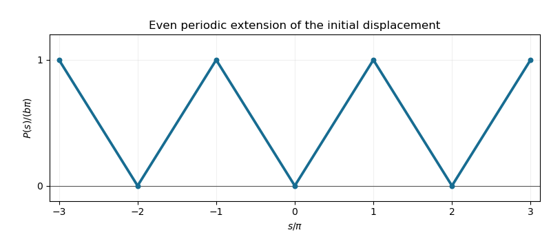
Even periodic extension of the initial displacement for the Neumann wave equation
. Retain the order of the noncommuting position operator and momentum operator. Using their commutator , expansion givesThus the two factorizations of the quantum harmonic oscillator are
Part (a) implies . Since , it follows thatFor an eigenfunction of the Hamiltonian with eigenvalue ,Thus is a ladder operator lowering the energy by , provided . The zero function is not an eigenfunction; in particular the ground state is annihilated by this operator. This qualification is essential for the later argument.
With the inner product , the assumed Hermiticity of and givesConsequently the adjoint relation isAs with the stated Hermiticity assumption, these identities concern wavefunctions in the appropriate operator domains. Square integrability alone does not guarantee that derivatives or multiplication by are square integrable; one may first work with smooth rapidly decaying wavefunctions, where integration by parts has no boundary term, and then use the operator domains.
Apply the adjoint operator identity of part (c) with and use part (a):For a nonzero eigenfunction, positivity of the norm in particular forces . Hence the requested norm isIt vanishes exactly at the ground-state energy.
The Hamiltonian of the quantum harmonic oscillator is the sum of two positive quadratic forms. For a nonzero eigenfunction in its domain,Thus . Part (d) supplies the stronger bound .
Start with a nonzero eigenfunction of energy and apply the lowering ladder operator repeatedly. Whenever the resulting wavefunction is nonzero, part (b) makes it an eigenfunction of energy . This cannot remain nonzero for every , since part (e) rules out negative energies. Let be the last nonzero member. Then , and part (d) forces its energy to be . Therefore every energy eigenvalue has the formThese levels actually occur: solving with gives the normalizable Gaussian . The raising operator increases the energy by , and . Repeated raising therefore produces a nonzero normalizable state at every listed level.
Use SI units and the Minkowski metric . Write , and the four-current , with Greek indices from to . The electromagnetic field tensor is the antisymmetric tensor whose components areIndices are raised and lowered with . Define the dual electromagnetic field tensor by , with . Then the covariant Maxwell equations areHere and are charge and current density, is the vacuum magnetic permeability, and . For example the equation gives , and the spatial equations give . With the stated dual convention, and ; the second tensor equation gives the two homogeneous Maxwell equations.
Contractions of Lorentz tensors have no free indices and are Lorentz scalars. The antisymmetry and the components in part (a) giveThus and are the two electromagnetic field invariants under proper Lorentz transformations. The second contraction uses the orientation-dependent epsilon tensor: strictly, is a pseudoscalar, changing sign under an improper transformation such as spatial parity. Under the boosts in this question it is invariant.
Articles were limited to the first 100 out of 122 total.
Articles by others on the same topic
There are currently no matching articles.