Past exam of the mathematics course of the year 1 of the natural sciences course of the University of Cambridge / 2007 / Paper 1

The factor theorem gives a factor $x-1$. Polynomial division and then factorization giveConsequently all three roots of a polynomial are

The chain rule for the cosine gives

The product rule and the derivative of the exponential function give

With the change of variables $u=3+2x$, $du=2dx$, an antiderivative isHere $C$ is the constant of integration.

Integration by parts with $u=\ln x$ and $dv=xdx$ givesThe remaining integral is $\frac{1}{2}\int xdx$.

Completing the square puts the equation of the circle in the formHence its centre is $(0,-3)$ and its radius is $2$.

This arithmetic series has $101$ terms, from $1$ to $201$. Thus

The geometric series has first term $1$ and common ratio $1/3$, whose absolute value is less than one. Therefore

On this parametric curve, $x=1$ permits $t=0$ or $t=-2$, but only $t=0$ also gives $y=0$. The chain rule gives the slopeAt the required point, $t=0$, so

The double-angle identity for the sine factors the equation as $2\cos \theta (\sin \theta -\cos \theta )=0$. The first factor gives $\theta =\pi /2$ in the specified interval; the second gives $\tan \theta =1$ and hence $\theta =\pi /4$. ThusKeeping the first factor avoids losing the solution where division by $\cos \theta$ would be invalid.

Call the centre of the circle $O$, the left endpoint on the diameter $A$, the point of tangency $T$, and the external intersection $E$. Since $OA=OT$ are radii, the isosceles triangle $AOT$ has equal base angles: $\angle OAT=\angle ATO=30^{\circ }$. Therefore $\angle AOT=120^{\circ }$, and, because $OA$ and $OE$ point in opposite directions, $\angle TOE=60^{\circ }$. The tangent to a circle $TE$ is perpendicular to the radius $OT$, so in the right triangle $OTE$,

Rationalizing a denominator by multiplying by $\sqrt{5}-1$ gives $2/(\sqrt{5}+1)=(\sqrt{5}-1)/2$. Consequently the sum inside the parentheses is $\sqrt{5}$, and the entire expression is

The function is nonnegative and satisfies ${\cos }^2(\pi -x)={\cos }^{2}x$. Its derivative is $-\sin (2x)$, so it decreases from $(0,1)$ to its minimum $(\pi /2,0)$ and then increases to $(\pi ,1)$. These three points all have horizontal tangent lines.

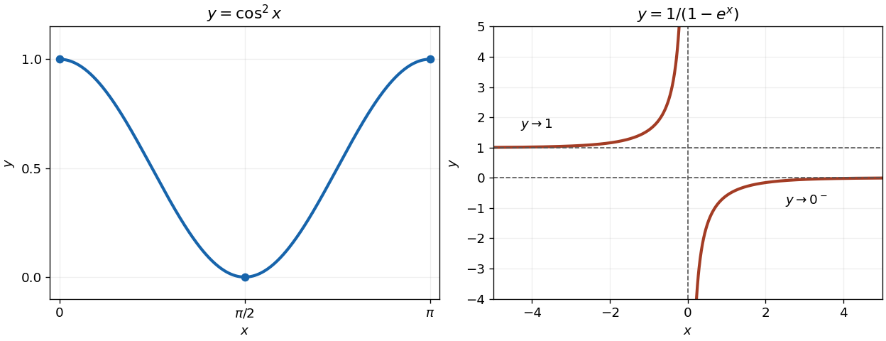
The denominator vanishes only at $x=0$, giving a vertical asymptote. Since $1-e^x=-x+O(x^2)$, the function tends to $+\infty$ from the left and $-\infty$ from the right. Its derivative isso each branch is increasing. The horizontal asymptotes are $y=1$ as $x\to -\infty$ and $y=0$ as $x\to +\infty$. The left branch lies above $1$; the right branch lies below $0$, as in the preceding figure.

If tangency occurs at $x_{\ast }$, the slope must satisfy both $k=2e^{2x_{\ast }}$ and $k{x}_{\ast }=e^{2x_{\ast }}$. Eliminating $k$ gives $2x_{\ast }=1$, so the tangent through the origin to an exponential curve has

The preceding tangent line calculation gives $x_{\ast }=1/2$ and $y_{\ast }=e^{2x_{\ast }}=e$. The point of tangency is

Because $\mathbf{b}\cdot \mathbf{x}$ is a scalar, applying the linear operator again givesThis is the first nontrivial case of the powers of a rank-one operator; its matrix is the outer product $\mathbf{a}{\mathbf{b}}^T$.

The vector triple product identity and $\mathbf{n}\cdot \mathbf{n}=1$ giveApply $H$ once more. The term parallel to $\mathbf{n}$ vanishes under its cross product with $\mathbf{n}$, leaving $H^3\mathbf{x}=-{\alpha }^3\mathbf{n}\times \mathbf{x}=-{\alpha }^{2}H\mathbf{x}$. The result includes $\alpha =0$.

The displayed power series is the matrix exponential $G=e^H$. From $H^3=-{\alpha }^{2}H$, its odd powers and nonconstant even powers sum separately:The scalar power series are $\sin \alpha /\alpha$ and $(1-\cos \alpha )/{\alpha }^2$, with continuous values $1$ and $1/2$ at zero. Substituting $H\mathbf{x}=\alpha \mathbf{n}\times \mathbf{x}$ and the preceding formula for $H^2\mathbf{x}$ yieldsThis is the Rodrigues rotation formula: the component parallel to $\mathbf{n}$ is fixed, while the perpendicular component undergoes a rotation through $\alpha$. For $\alpha =0$ the linear operator is the identity operator.

Using the principal complex logarithm, $\mathrm{Log}i=i\pi /2$ and $\mathrm{Log}(-e)=1+i\pi$. Thus the values and their real parts and imaginary parts areFor the final row, first calculate $i^i=e^{-\pi /2}$ and only then raise this positive real number to the power $i$. Treating nested powers as ordinary real powers would ignore the branching of complex exponentiation.

If all branches are requested, $\sqrt{i}$ also has the negative of its principal value, and the complex logarithm of $-e$ is $1+i(\pi +2\pi k)$. Allowing nonprincipal logarithms of the positive base $2$ gives $e^{-2\pi k}{e}^{i\ln 2}$. Finally, all values of $(i^i{)}^i$ are $-i{e}^{-2\pi m}$, for integers $k,m$ as appropriate. These alternatives do not alter the principal-value table.

Euler's formula givesCubing the expression for the sine, and grouping the $e^{3ix}$ and $e^{-3ix}$ terms, givesThe required equation therefore becomes $\sin x(1-4{\sin }^{2}x)=0$. The complete real solution set is

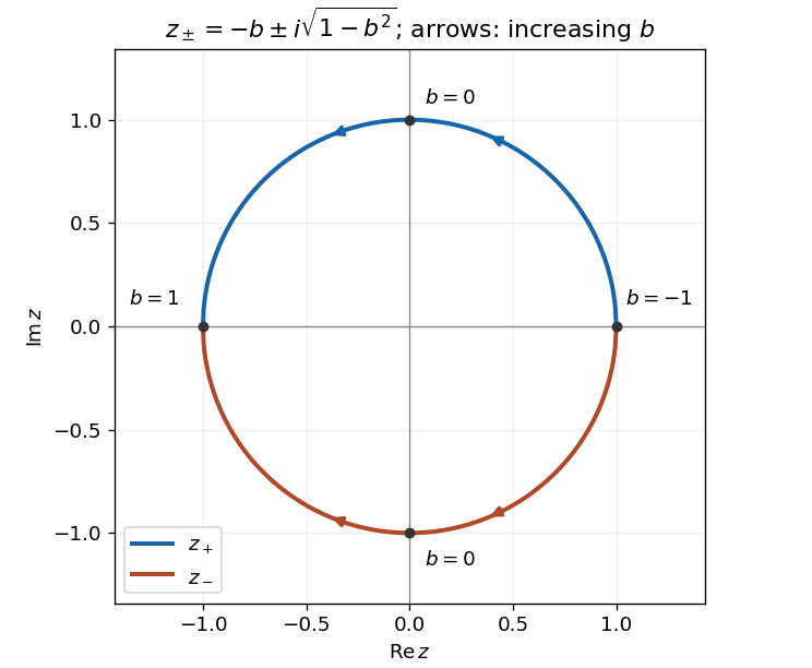
The quadratic formula gives $z=-b\pm \sqrt{b^2-1}$. For $-1\le b\le 1$, write this asEach root of a polynomial has modulus $1$, since $b^2+(1-b^2)=1$. As $b$ increases from $-1$ to $1$, the upper root traverses the upper unit semicircle from $1$ to $-1$, and the lower root traverses the lower semicircle in the opposite angular direction. At $b=-1$ the roots coincide at $1$; at $b=1$ they coincide at $-1$. For intermediate $b$ they are complex conjugates.

Since the derivative of the arctangent is $1/(1+x^2)=1-x^2+O(x^4)$ near zero, termwise integration givesThe integration constant is zero because $\arctan 0=0$.

The expression in the PDF is $1/a^x-1$, with the subtraction outside the fraction. Using the exponential series with $a^{-x}=e^{-x\ln a}$ givesFor $a>0$, $a\ne 1$, these are the first two nonzero terms. If $a=1$, the function is identically zero, so there are no nonvanishing terms.

The square is on the cosine: near zero, $\ln ({\cos }^{2}x)=2\ln (\cos x)$. Substituting $\cos x=1-x^2/2+x^4/24+O(x^6)$ into the logarithmic series givesTherefore

Since $g(0)=0$, only the first three positive powers of $g$ contribute through degree three. The composition coefficients of power series follow by using $g^2=g_1^2{x}^2+2g_1{g}_2{x}^3+O(x^4)$ and $g^3=g_1^3{x}^3+O(x^4)$ in $f_0+f_{1}g+f_2{g}^2+f_3{g}^3+\cdots$. HenceHere $f_m$ and $g_m$ are coefficients of the power series, rather than raw derivatives; their definitions already contain any factorial factors.

The exponential series proves normalization of a probability distribution:Let $M$ and $F$ count the two labels. Conditional on $N=M+F=k+l$, independent labeling gives a binomial distribution, so the joint probability mass function isEach bracket is a normalized Poisson distribution. Summing over $l\ge 0$ therefore givesThe factorization also proves that $M$ and $F$ are independent random variables. This is Poisson thinning; the phrase about ignoring the other count refers to taking a marginal distribution, rather than fixing that count.

Let $D$, $C$, and $V_0$ denote the three disjoint categories, and $+$ or $-$ the test result. The law of total probability givesTo calculate the requested conditional probability, first combine the two categories with the virus. Their joint negative-test probability is $0.1(0.05)+0.2(0.1)=0.025$, whereas $\mathbb{P}(-)=1-0.31=0.69$. Bayes' theorem therefore givesThese numbers use the specified population proportions and test probabilities; the negative result reduces the initial combined proportion $0.3$ to about $3.62\%$ within this model.

Writing the differential one-form as $Mdx+Ndy$, its coefficients satisfy $M_y=e^y\cos x=N_x$. It is an exact differential form, with potential $F=(1+e^y)\sin x$, becauseThe implicit solution is therefore

On the real domain $y>0$, $M=y(x^2+\ln y)$ and $N=x$ have $M_y=x^2+\ln y+1$ and $N_x=1$, so this differential one-form is not exact. An integrating factor for a differential one-form is $\mu =1/y$, which is nonzero on this domain. Multiplication givesHence the implicit solution is

On the interval $x>-1$ containing the initial condition, division by $1+x$ gives a linear ordinary differential equation with integrating factor $(1+x{)}^{-3}$. ConsequentlyThe initial value gives $C=1$. ThusThis polynomial also satisfies the original equation at $x=-1$ and gives an extension to all real $x$. The initial value problem is uniquely determined on $x>-1$; the vanishing leading coefficient at $-1$ does not ensure unique continuation to its left.

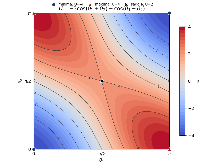
Put $S={\theta }_1+{\theta }_2$ and $D={\theta }_1-{\theta }_2$. The gradient has components $3\sin S+\sin D$ and $3\sin S-\sin D$, so a stationary point requires $\sin S=\sin D=0$. In the closed square, $S\in [0,2\pi ]$ and $D\in [-\pi ,\pi ]$, and the compatible possibilities are precisely the four corners and $(\pi /2,\pi /2)$.

The Hessian matrix isIts eigenvectors $(1,1)$ and $(1,-1)$ have eigenvalues $6\cos S$ and $2\cos D$. The second-derivative test gives the following classification:

The corner classifications also hold for the smooth extension beyond the square, and hence for the restricted region. The global bounds $-4\le U\le 4$ show that the stated minima and maxima are global within it. The central point has opposite curvature along the two diagonal directions.

The region is $0\le y\le 1$, $2y\le x\le 2$. Reversing the order describes the same triangle as $0\le x\le 2$, $0\le y\le x/2$. Since the integrand is continuous on this compact region, Fubini's theorem permitsThe new inner integral introduces the factor $x$ needed for the change of variables $u=x^2$.

In cylindrical coordinates the spherical cap has $1<z<\sqrt{2}$, $0<r<\sqrt{2-z^2}$ and $0<\theta <2\pi$. Its mass density is $kz$ and the volume element is $rdrd\theta dz$. ThereforeThis is the mass of a spherical cap with height-proportional density with $R=\sqrt{2}$ and $c=1$.

For its curved surface area, write $z=\sqrt{2-r^2}$ with $0\le r\le 1$. The surface integral of one becomesIt agrees with the curved area of a spherical cap, $2\pi Rh$, for $h=\sqrt{2}-1$. The planar closing disk is not part of the requested curved surface.

False. Take the diagonal matrix $A=\mathrm{diag}(1,2)$ and its eigenvectors $\mathbf{x}=(1,0{)}^T$, $\mathbf{y}=(0,1{)}^T$. Their sum $(1,1{)}^T$ is mapped to $(1,2{)}^T$, which is not a scalar multiple of that sum. More generally, $A(\mathbf{x}+\mathbf{y})=a\mathbf{x}+c\mathbf{y}$ need not have the form $\lambda (\mathbf{x}+\mathbf{y})$ when $a\ne c$.

True. By linearity, $(A+B)\mathbf{x}=A\mathbf{x}+B\mathbf{x}=(a+b)\mathbf{x}$. Since $\mathbf{x}\ne 0$, it is an eigenvector of $A+B$ with eigenvalue

True. Applying the matrices in order gives $AB\mathbf{x}=A(b\mathbf{x})=ab\mathbf{x}$. The eigenvalue isThis conclusion only uses the shared eigenvector; it does not require $A$ and $B$ to commute on other vectors.

If $A\mathbf{v}=\lambda \mathbf{v}$ for a nonzero eigenvector, then $A^2\mathbf{v}={\lambda }^2\mathbf{v}=A\mathbf{v}=\lambda \mathbf{v}$. Thus $\lambda (\lambda -1)=0$, soBoth values need not occur: the zero matrix has only $0$, and the identity matrix only $1$. More precisely, an idempotent linear map whose rank of a linear map is $r$ has $r$ copies of $1$ and $n-r$ copies of $0$. Indeed, its image of a linear map and kernel of a linear map form a direct sum, giving an eigenbasis without assuming an orthogonal projection.

On an eigenvector of $A$ with eigenvalue $\lambda$, the linear operator $B=I-A$ has eigenvalue $1-\lambda$. ThereforeThe multiplicities are exchanged: if the matrix rank of $A$ is $r$, then $B$ has $n-r$ copies of $1$ and $r$ copies of $0$. Again, a value with zero multiplicity is absent.

Computing the characteristic polynomial with the convention $\det (\lambda I-H)$ givesThus the three eigenvalues areThey can also be checked directly on the respective eigenvectors $(1,0,-1{)}^T$, $(1,-1,1{)}^T$, and $(1,2,1{)}^T$.