Past exam of the mathematics course of the year 2 of the natural sciences course of the University of Cambridge / 2022 / Paper 1

Let $\rho =\sqrt{x^2+y^2}=uv$. The condition $u\le v$ gives $z\le 0$. On the outer coordinate surface $v=1$, elimination of $u$ gives $z=({\rho }^2-1)/2$. On $u=v$, the surface is the plane $z=0$, with $\rho =u^2\le 1$. Thus the closure of the body isIt is a solid circular cap bounded below by an elliptic paraboloid of revolution and above by the unit disk in $z=0$. Its vertex is $\boxed{(0,0,-1/2)}$, its height is $\boxed{1/2}$, and its rim is the circle $\boxed{x^2+y^2=1,z=0}$. The symmetry axis is the $z$ axis. The coordinate surface $u=0$ maps to that axis rather than to an additional two-dimensional boundary. These are parabolic coordinates.

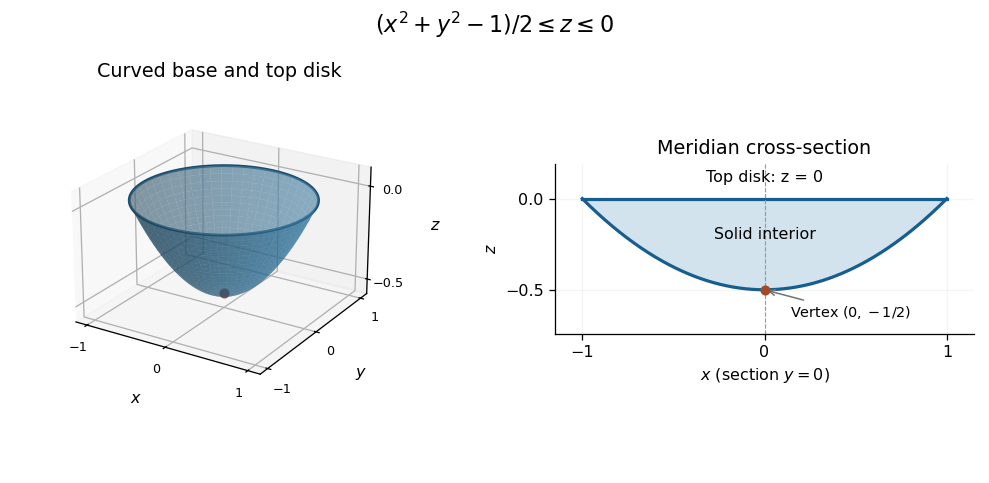
Differentiate the position vector with respect to the three coordinates to obtain the coordinate basis vectors:The chain rule gives $d\mathbf{x}={\mathbf{h}}_{u}du+{\mathbf{h}}_{v}dv+{\mathbf{h}}_{\varphi }d\varphi$. The scale factors of orthogonal coordinates are the corresponding norms:Direct dot products give ${\mathbf{h}}_u\cdot {\mathbf{h}}_v=uv-uv=0$, ${\mathbf{h}}_u\cdot {\mathbf{h}}_{\varphi }=0$, and ${\mathbf{h}}_v\cdot {\mathbf{h}}_{\varphi }=0$. Thus the parabolic coordinates are orthogonal wherever the coordinate vectors are nondegenerate. Their degeneracy on $uv=0$ is the usual axis degeneracy of the azimuthal coordinate.

The Jacobian determinant is the oriented scalar triple product of the three coordinate basis vectors:Here ${\mathbf{h}}_u\times {\mathbf{h}}_v=(u^2+v^2)(-\sin \varphi ,\cos \varphi ,0)$, soThe sign is nonnegative on the stated range, and the absolute Jacobian determinant also equals $h_u{h}_v{h}_{\varphi }$ as expected for orthogonal coordinates.

Since $\mathbf{F}=\nabla \Omega$, its divergence is the Laplacian of $\Omega$:The divergence theorem changes the outward flux through the whole closed boundary into $I={\int }_V(6x+4z)dV$. Rotational symmetry makes the $x$ term vanish. With $z=(u^2-v^2)/2$ and the Jacobian determinant from part (c),Both the curved face and the top disk are included in this surface integral through the divergence theorem.

Remove the common nonzero factor $e^{-i\omega t}$ and expand in the small parameter $ϵ$. To first order, the modified Laplacian contributes only its $y$ derivatives: its $x$ derivative term has the extra factor ${ϵ}^2$. The regular perturbation expansion therefore givesThus the two residuals are $P+ϵQ+O({ϵ}^2)$ and $R+ϵS+O({ϵ}^2)$, respectively. Subscripts after a comma denote partial derivatives. We retain $\omega \ne 0$, as appropriate to the oscillatory wave and the elimination below.

Insert the proposed leading relation into the two zeroth-order residuals. It givesand, since $b_{0,y}=-i{\psi }_{0,yy}$,Hence $\boxed{b_0=-i{\psi }_{0,y}⟹P=R=0}$. The same relation is forced by $P=0$ when $\omega \ne 0$; its $y$ derivative then automatically gives $R=0$.

The first-order condition $Q=0$, combined with $b_0=-i{\psi }_{0,y}$, givesDifferentiate this expression with respect to $y$ and insert it into $S=0$. The ${\psi }_1$ terms cancel, leavingThus the compatibility partial differential equation isIt is exactly ${\partial }_y(2{\psi }_{0,x}+i{\psi }_{0,yyy})=0$. Integrating with respect to $y$ therefore giveswhere the integration constant may be any function of $x$. Conversely, differentiating this last equation with respect to $y$ recovers the compatibility equation.

For separation of variables matching the boundary Fourier mode, take ${\psi }_0=X(x)e^{iky}$ with $X(0)=1$. Because ${\partial }_y^3{e}^{iky}=-i{k}^3{e}^{iky}$, the reduced ordinary differential equation isThereforeThe decay of a Fourier mode in a third-order spatial evolution equation requires a sign check: this satisfies the requested limit at positive infinity precisely when $\boxed{k>0}$. For $k=0$ it remains identically one, while for $k<0$ its amplitude grows exponentially. Hence for those nonpositive values there is no separated solution meeting both prescribed boundary conditions; the printed assumption that $k$ is merely real needs this additional restriction for decay.

The homogeneous equation is a Cauchy-Euler equation. With the power-law ansatz $y=x^r$ on $x>0$, its indicial equation isThus $r=(1-\alpha )/2$ is a repeated indicial root. The two independent solutions are $x^r$ and $x^r\log x$, givingTheir Wronskian, with $W=y_1{y}_2^{\prime }-y_1^{\prime }{y}_2$, is $x^{2r-1}=x^{-\alpha }\ne 0$, verifying linear independence.

Choose the causal Green function convention $L_{x}G(x,\xi )=\delta (x-\xi )$ for each source point $\xi >0$, with $G(x,\xi )=0$ when $x<\xi$. This automatically gives the two zero-origin limits. The kernel is continuous at $x=\xi$, and integrating its equation across the source requires the unit derivative jump ${\partial }_{x}G({\xi }^{+},\xi )-{\partial }_{x}G({\xi }^{-},\xi )=1$.

For $x>\xi$, the homogeneous basis from part (a) gives a continuous kernel proportional to $x^r\log (x/\xi )$. Its derivative at $x=\xi$ is ${\xi }^{r-1}$, so the normalization is ${\xi }^{1-r}$. Hence the causal Green function for a repeated-root Euler operator isThe same formula follows from $[y_1(\xi )y_2(x)-y_2(\xi )y_1(x)]/W(\xi )$ on the right of the source, with $W(\xi )={\xi }^{-\alpha }$.

The singular endpoint matters for uniqueness. If $\alpha <-1$, then $r>1$, and both $x^r$ and $x^r\log x$, together with their first derivatives, vanish at zero. Adding any source-dependent linear combination of these homogeneous solutions to $G$ preserves the two stated origin conditions. Thus those conditions alone do not determine a unique Green's function in that parameter range. The causal requirement used here selects the displayed kernel. For $\alpha \ge -1$ no nonzero homogeneous solution satisfies both zero-origin limits, so this ambiguity is absent.

Using the causal Green's function,Put $\xi =xs$. Since $\alpha >-5$ is equivalent to $r<3$, the improper integral converges and givesThe elementary identity ${\int }_0^1{s}^{p-1}(-\log s)ds=1/p^2$ follows by differentiating ${\int }_0^1{s}^{p-1}ds=1/p$ for $p>0$. Direct substitution checks $L(x^3)=(\alpha +5{)}^{2}x/4$, and the displayed solution and its first derivative vanish at zero.

To give all solutions allowed by the printed boundary conditions, retain the singular-endpoint qualification from part (b):Thus the causal integral gives a particular member of a two-parameter family in the first range and the unique solution in the second.

For integrable functions $f,g$, Fubini's theorem justifies exchanging the two integrals in the Fourier transform of the convolution. Set $s=x-t$ to obtainThis proves the convolution theorem with the stated normalization:

Direct evaluation gives the first Fourier transform:For the even triangular function, the odd sine part integrates to zero. Two elementary integrations by parts or one evaluation of the cosine integral giveThe values at zero are the respective areas, agreeing with the removable limits. Therefore $\tilde{g}={\tilde{f}}^2$. By the convolution theorem and uniqueness of the Fourier transform,There is also a direct interpretation: the convolution is the length of overlap of the intervals $(-1/2,1/2)$ and $(x-1/2,x+1/2)$, giving exactly that triangular profile.

The Parseval identity for this Fourier transform convention isApply it to $h=g$. Its squared norm is $2{\int }_0^1(1-x{)}^{2}dx=2/3$, soUnder $k=2x$, the last integrand times $dk$ becomes $2{\sin }^{4}xdx/x^4$. ConsequentlyThe integrand has continuous value $1$ at zero and decays integrably at infinity, so this is an ordinary convergent improper integral.

A square matrix is a diagonalizable matrix over the chosen field when there are an invertible matrix $P$ and a diagonal matrix $D$ such that $A=PD{P}^{-1}$. If $v_j$ is column $j$ of $P$ and $D_{jj}={\lambda }_j$, the identity $AP=PD$ gives $A{v}_j={\lambda }_j{v}_j$. Invertibility makes these $n$ columns linearly independent eigenvectors.

Conversely, put $n$ linearly independent eigenvectors in the columns of $P$ and their eigenvalues in $D$. Then $P$ is invertible and $AP=PD$, givingRepeated eigenvalues are allowed; the requirement is a complete eigenbasis, not distinctness of the eigenvalues.

A single eigenbasis works for every choice of the parameters. The columns $v_1=(1,0,0{)}^T$, $v_2=(1,1,0{)}^T$, $v_3=(1,1,1{)}^T$ satisfyThey are linearly independent because their column matrix has determinant one. Thus the diagonalization isThis formula includes all coincidences among $a,b,c$, so no special repeated-eigenvalue cases need separate bases.

The diagonalization in part (b) gives $M^k=P\mathrm{diag}(a^k,b^k,c^k)P^{-1}$. HenceSufficiency follows from the scalar powers tending to zero; necessity also follows immediately from the diagonal entries of $M^k$. Under these conditions the matrix geometric series converges, and its sum isWriting $A_0=1/(1-a)$, $B_0=1/(1-b)$ and $C_0=1/(1-c)$, all entries are explicitlyFor example, $B_0-A_0=(b-a)/[(1-a)(1-b)]$ and $C_0-B_0=(c-b)/[(1-b)(1-c)]$. These expressions remain valid when parameter values coincide.

Expand the quadratic form of this Gram matrix:For $\mathbf{c}\ne 0$, linear independence of the real vectors implies ${\sum }_i{c}_i{\mathbf{x}}_i\ne 0$, so its squared Euclidean norm is strictly positive. Thusproving the positive definiteness of a Gram matrix in the independent-vector case.

A skew-Hermitian matrix satisfies $A^{†}=-A$, where $†$ denotes the conjugate transpose. If $Av=\lambda v$ with $v\ne 0$, thenSince $v^{†}v>0$, this gives $\boxed{\overline{\lambda }=-\lambda ,\text{ so }\lambda \in i\mathbb{R}}$.

A unitary matrix satisfies $U^{†}U=U{U}^{†}=I$. It preserves the Hermitian inner product and norm. Thus if $Uv=\mu v$,and therefore $\boxed{|\mu |=1}$. Zero is allowed among the purely imaginary eigenvalues in the first statement, but not among the unitary eigenvalues.

Let $A{v}_i={\lambda }_i{v}_i$ and $A{v}_j={\lambda }_j{v}_j$. The skew-Hermitian matrix property giveswhere the last equality uses part (a). Distinct eigenvalues therefore imply $\boxed{v_i^{†}{v}_j=0\text{ for }i\ne j}$. Normalize each eigenvector to length one. Since there are $n$ distinct eigenvalues, these vectors form an orthonormal basis.

Put them in the columns of $U$. Then $U$ is a unitary matrix and $AU=UD$, so

To avoid confusing the diagonalizing matrix with the exponential, write $A=WD{W}^{†}$ from part (b). The convergent matrix exponential series givesEach ${\lambda }_j$ is purely imaginary, so $|e^{{\lambda }_j}|=1$. The diagonal exponential is therefore a unitary matrix, andHence the matrix called $U=\exp (A)$ in this part is unitary. The series identity $(e^A{)}^{†}=e^{A^{†}}=e^{-A}$ gives the same conclusion directly and also covers repeated eigenvalues.

Since both real matrices are antisymmetric, $A^{†}=-A$ and $B^{†}=-B$. Thus $U^{†}=-A+iB$. Expand the two unitary identities:Subtracting and adding give $\boxed{AB=BA,A^2+B^2=-I}$. Because $A$ has simple eigenvalues, each of its complex eigenspaces is one-dimensional. Commutation makes each one invariant under $B$: if $Av=av$, then $A(Bv)=a(Bv)$. Hence $Bv=bv$ for some scalar $b$. The complete eigenbasis of $A$ is therefore a common eigenbasis, which also diagonalizes $U$.

The skew-Hermitian decomposition of a unitary matrix is explicit:If $Uv=uv$, unitarity gives $U^{†}v=u^{-1}v=\overline{u}v$. ConsequentlyEquivalently, for $u=e^{i\theta }$ the paired eigenvalues are $\boxed{a=i\sin \theta ,b=-i\cos \theta }$. The hypotheses can only occur in even dimension: $U^T=-U$ and $U$ is invertible, whereas an odd-dimensional skew-symmetric matrix has zero determinant.

The Cauchy-Riemann equations are $\boxed{u_x=v_y,u_y=-v_x}$. They give the gradient identityAt a regular intersection, where $f^{\prime }(z)\ne 0$, the two nonzero gradients are normal vectors to the two level sets, so their tangent directions are perpendicular. This is the orthogonality of regular real and imaginary level curves.

The regularity qualification is necessary: $|\nabla u|=|\nabla v|=|f^{\prime }|$, so at a critical point both normals vanish and the curves need not have unique tangents. For example $f=z^2$ gives diagonal lines for $u=0$ and coordinate axes for $v=0$, all meeting at the origin. Thus the conclusion is $\boxed{\text{right-angle intersection wherever }{f}^{\prime }(z)\ne 0}$, rather than an unrestricted claim at critical points.

Write $g=u+iv$ and let its constant modulus be $C$. If $C=0$, then $g=0$. For $C>0$, differentiating $u^2+v^2=C^2$ with respect to $x$ and $y$, then applying the Cauchy-Riemann equations, givesThusThe coefficient matrix has determinant $-(u^2+v^2)=-C^2\ne 0$, forcing $u_x=v_x=0$. The Cauchy-Riemann equations then also give $u_y=v_y=0$. Therefore $u,v$ are constant on a connected domain andThis proves the constant-modulus holomorphic function result. If a domain is disconnected, the conclusion applies separately to each connected component.

The zeros of $\sin z$ are $z=n\pi$ for $n\in \mathbb{Z}$, all simple, and $\cos (n\pi )=(-1{)}^n\ne 0$. Hence the finite singularities of $\cot z$ are exactlyLocally $\cot z\sim 1/(z-n\pi )$, so each pole has residue $1$.

For $z\ne 0$, singularities occur when $1/z=n\pi$, with $n\ne 0$. Each is a simple pole, since the substitution has nonzero derivative there:More explicitly, $1/z-n\pi \sim -(z-z_n)/z_n^2$, so $\cot (1/z)\sim -z_n^2/(z-z_n)$ and its residue is $-1/(n^2{\pi }^2)$.

These poles accumulate at zero. Consequently $\boxed{z=0\text{ is a non-isolated singularity}}$. The removable/pole/essential classification for isolated singularities cannot be applied at that accumulation point; it is not an isolated essential singularity.

At every $z=n\pi$, the inner function has a simple pole, with $\cot z=1/(z-n\pi )+h(z)$ for analytic $h$. ThusThe first factor is analytic and nonzero, while the second has infinitely many negative powers in its Laurent series. Therefore, by the exponential of a pole is an essential singularity result,At all other finite points the composition is analytic, so there are no additional finite singularities.

Set $w=z-1$. Partial fraction decomposition givesExpand both terms as geometric series:The two bracketed terms are complex conjugates. Using $1\pm i=\sqrt{2}{e}^{\pm i\pi /4}$ produces the required real coefficients:The initial terms are $1-\frac{1}{2}{w}^2+\frac{1}{2}{w}^3-\frac{1}{4}{w}^4+\cdots$. The nearest singularities are the simple poles $z=\pm i$, both at distance $\sqrt{2}$ from the center. Hence the Taylor series has

A finite point $x_0$ is an ordinary point when the normal-form coefficients $p,q$ are analytic at $x_0$. Then arbitrary values $y(x_0),y^{\prime }(x_0)$ determine a convergent Taylor series, and two independent choices give two linearly independent local analytic solutions.

A singular point is a regular singular point when $(x-x_0)p(x)$ and $(x-x_0{)}^{2}q(x)$ extend analytically to $x_0$. The Frobenius method then provides at least one solutionwith a locally convergent analytic factor and an exponent fixed by the indicial equation. If its two indicial roots differ by a noninteger, there are two independent Frobenius solutions. For integer-separated roots a second solution may include a logarithm; a repeated root gives a Logarithmic Frobenius solution accompanying the single pure series. Such solutions need not be finite or ordinary Taylor series at the singular point.

Expanding the derivative and dividing by $1-x$ givesThe only finite singular point is $\boxed{x=1}$. There $(x-1)p(x)=1$ and $(x-1{)}^{2}q(x)=c^2(x-1{)}^2-\lambda (x-1)$ are analytic, so it is a regular singular point. At infinity the coefficient of $y$ tends to $c^2\ne 0$, giving an irregular singular point after reciprocal substitution; the finite classification is independent of $\lambda$.

Put $t=1-x$ and $Y(t)=y(x)$. The differential equation becomesSubstitute the Frobenius solution $Y=t^{\sigma }{\sum }_{n\ge 0}{a}_n{t}^n$. The lowest power has coefficient ${\sigma }^2{a}_0$, soEquating successive coefficients gives, with $a_{-1}=0$,Thus $a_0\ne 0$ is the only free coefficient: $a_1=-\lambda a_0$, $a_2=({\lambda }^2-c^2)a_0/4$, and so on. Since every denominator is nonzero, there is exactly one independent pure Frobenius solution of this form. The repeated root supplies no second free coefficient; the other solution is logarithmic, as parts (iii) and (iv) demonstrate.