Options I, Honour School of Mathematics; Friday 23 June 2006, 9.30am–12.30pm. The complete nine-page source was supplied in the disclosed past-papers archive, member “FOI-20210708-1 - Data/4303 (6).pdf”, through the original request. The full source is privately transcribed. No exact worked-answer advertisement was found in the bounded availability check.
Write the group action as . A right group action satisfies and . Its orbit and stabilizer areThe identity belongs to . If , then , so . Also implies , so . Thus is a subgroup.
For the orbit-stabilizer theorem, the map , , is onto, andIts fibers are precisely the right cosets , each containing elements. Counting these disjoint fibers givesFor the symmetric group , the six subgroups areThe group action has four orbits: each of , , and is fixed, while the three order-two subgroups form one orbit. Here an orbit is a collection of subgroups, rather than a collection of individual permutations.
A field extension is finite when , regarded as a vector space over , has finite dimension. Its degree of a field extension isThus a finite basis means that every is uniquely expressible as with coefficients .
Since is an -vector subspace of the finite-dimensional vector space , it has a finite -basis . Any finite -spanning set for also spans over , so choose a finite -basis of .
Every can be expanded first in the and then in the , showing that the products span over . If with , independence of the over gives for every ; independence of the then gives every . The products form an -basis, proving the tower law for field extensions:
Put . The tower law for field extensions shows that both and divide . Since are coprime, their product divides , so .
The minimal polynomial of over has degree and is still an annihilating polynomial over . The minimal polynomial over divides it, soThe upper and lower bounds agree:Coprimality is the step forcing the lower bound to equal the product; without it the two generated fields can overlap substantially.
Use the agreed text encoding to split the plaintext into integer blocks . RSA encrypts each block by modular exponentiation:Because is a product of distinct primes, its Euler totient function is . The inverse exponent follows fromThus a decryption exponent is 275, and the three recovered blocks areTo check every block, including blocks not coprime to the modulus, reduce modulo each prime. If is nonzero modulo 29, Fermat's little theorem gives because ; if it is zero the equality is immediate. The same argument works modulo 37 because . The Chinese remainder theorem then gives the equality modulo 1073. Finally reverse the agreed text encoding. The symbols are unspecified, so there are no numerical message blocks to evaluate further.
The Gaussian function is continuous and hence Lebesgue measurable. For , , and thereforeThe right side has finite Lebesgue integral: its first term has integral 4 and the second is Lebesgue integrable by hypothesis. The comparison principle for the Lebesgue integral says that a measurable nonnegative function dominated by an integrable function has finite integral. Consequently the Gaussian function is Lebesgue integrable.
A real measurable function is Lebesgue integrable precisely when the integral of its absolute value is finite. For every integer , on one has and . ConsequentlyThe intervals have disjoint interiors. Countable additivity of the nonnegative Lebesgue integral, or the monotone convergence theorem applied to their finite unions, givesThe harmonic series diverges, so the function is not Lebesgue integrable. Cancellation between adjacent oscillations cannot give absolute integrability.
The annulus is open and hence Lebesgue measurable; multiplying its indicator by the continuous Gaussian gives a measurable function. It is bounded by the indicator of , whose Lebesgue integral is . Thus it is Lebesgue integrable by comparison.
Use the change of variables formula with polar coordinates , . Removing one radial cut makes this a smooth one-to-one coordinate map; the cut is a null set and does not affect the integral. The absolute Jacobian determinant is . By Fubini theorem,The antiderivative is , which also makes the sign of the answer transparent.
In a metric space, a Cauchy sequence has arbitrarily small distances between all sufficiently late terms:This condition compares terms to each other and does not assume that a limit exists in the space.
A sequence converges to whenThe phrase convergent sequence requires the limit to belong to the stated metric space; convergence in a larger ambient space alone does not suffice.
A complete metric space is a metric space in which every Cauchy sequence converges to a point of that space.
Now let be complete in the induced metric. If , choose with . The sequence converges to in , so is a Cauchy sequence. Completeness of supplies a limit . Uniqueness of limits in a metric space gives , hence . Therefore a complete metric subspace is closed.
Completeness does not imply sequential compactness. In the complete space , the sequence has no convergent subsequence: a subsequence has strictly increasing indices , so and is unbounded, whereas every convergent real sequence is bounded.
A topological space is connected when it cannot be written as the union of two disjoint nonempty open sets. Equivalently, the only subsets that are simultaneously open and closed are the empty set and the whole space. For a subset, connectedness refers to its subspace topology.
True. Suppose were a separation into nonempty relatively open sets. Intersecting with gives a separation unless all of the connected set lies on one side; similarly all of lies on one side. A point of forces both to lie on the same side. The other side would then be empty, a contradiction. Hence is connected.
False. Take and . Both complements are disconnected: their negative and positive halves form a separation. Butis path-connected, hence connected. To see path connectedness directly, move any nonzero point radially to its normalization on the unit circle; join the two normalized points by a circular arc; then reverse the radial path for the second point. Every segment of this path avoids the origin. Thus disconnected coordinate complements do not force a disconnected complement of their product.
False. In , takeThen and are connected. Nevertheless is disconnected: and are disjoint nonempty relatively open sets partitioning . For instance, intersecting with and produces this separation. The endpoint missing from is supplied by , so the union becomes connected without forcing itself to be connected.
The rows of the Jacobian matrix are . Rank means precisely that these gradients are linearly independent. The Lagrange multiplier condition is that real numbers exist withGeometrically, is perpendicular to the tangent space of the constraint level set, whose tangent vectors form . The full-rank hypothesis ensures this level set is a smooth local constraint manifold.
The constraint set is compact, so the continuous objective attains a maximum and minimum. The two constraint gradients are nonzero and supported on separate coordinates, so they are linearly independent everywhere on it. The Lagrange multiplier equations areBoth positive and negative values occur. At a maximizing or minimizing point the objective is therefore nonzero, so , , and both are nonzero. The equations imply , , and . The constraints then give , .
Consequently, writing , the complete list of extrema isFor an independent global check, Cauchy-Schwarz inequality gives , with equality exactly at the displayed points.
Let be a smooth variation with . Assuming the usual continuous second derivatives of , stationarity of the functional under gives its first variationIntegration by parts removes the derivative of ; its boundary term vanishes because the endpoint values are fixed. Thusfor every such variation. The fundamental lemma of the calculus of variations implies the Euler-Lagrange equation .
For arc length, , soThe function is strictly increasing; hence is constant. With endpoints and , , the extremal isIt is also the global shortest curve: integrating the unit displacement vector dotted with the curve velocity gives the endpoint distance, which is at most the integrated speed by Cauchy-Schwarz inequality; the straight segment attains equality. A vertical segment is described parametrically or after rotating axes, since it cannot be represented by on a nontrivial horizontal interval.
For a holonomic conservative system the Lagrangian is , the difference between kinetic energy and potential energy. The Euler-Lagrange equations areIf , this gives for the generalized momentum . Such a coordinate is a cyclic coordinate.
In cylindrical coordinates the squared speed is . The holonomic constraint gives , while gravity has potential energy . ThereforeThere is no explicit dependence, so is a cyclic coordinate andThis is angular momentum about the vertical symmetry axis. At the polar angle is singular, but the Cartesian angular momentum remains well defined and has the same conserved value.
In SI units, Gauss's law for a closed surface with outward unit normal vector isSpherical symmetry and the absence of an imposed external field make the electric field radial, . For (with the physical radius ),Outside the charge distribution this becomes . Applying Gauss's law on spheres givesBoth formulas agree at , and the first tends to zero at the origin. Thus the total charge is . Negative reverses the field direction. If the radius is zero the distribution vanishes; a negative value of gives no nonnegative-radius support under the printed piecewise inequalities and likewise gives the zero distribution.
For a twice continuously differentiable stream function, equality of mixed derivatives givesThis is the incompressible flow condition in two dimensions. A streamline is a curve whose tangent at each regular point is parallel to the instantaneous velocity field. Parameterize it by . The chain rule yieldsTherefore the stream function is constant on each streamline. This proof includes arbitrary regular parametrizations; at a stagnation point the velocity vanishes and the usual tangent direction is not determined.
The complex potential of a two-dimensional potential flow is , soFor , a nonzero level isThus the streamlines are circles tangent to the horizontal axis at the excluded singular origin, with centers on the vertical axis. Each circle has the origin removed. The zero level is the horizontal axis without the origin, whose positive and negative rays are separate streamlines. Since is nonzero away from the origin, no other stagnation points intervene. For the flow vanishes everywhere off the origin, so the circle description is replaced by the degenerate zero-velocity field.
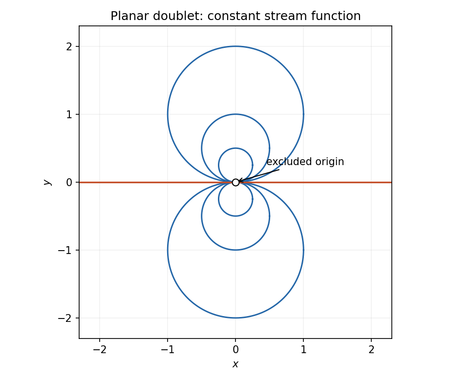
Streamlines of a planar doublet
. Circles tangent at the excluded origin and the two zero-level horizontal rays; the drawing uses positive doublet strength. Details.
The stream function gives and . Its scalar vorticity isFor this does not vanish on any nonempty open region of the plane. A holomorphic complex potential of a two-dimensional potential flow would produce an irrotational flow there. Equivalently, its imaginary part would be a harmonic function, whereas . Thus no complex potential exists on any nonempty open region for this flow; vanishing vorticity only along the vertical line does not provide a two-dimensional domain.
Start from the uniform-flow complex potential of a two-dimensional potential flow . Milne-Thomson's circle theorem adds the image doublet , yielding constant stream function on . Add a line vortex with positive counterclockwise circulation :Indeed, on the uniform-flow and doublet terms sum to the real number , while the vortex has imaginary part , also constant. Thus the cylinder is a streamline and satisfies the impermeability condition. The vortex velocity is in the counterclockwise direction. Although the potential is multivalued when , its velocity is single-valued.
Differentiate and locate the coefficient of in the square:For the counterclockwise contour in the printed Blasius force theorem, the residue theorem gives . ConsequentlyThese are force components per unit cylinder length; with the stated circulation convention the lift is downward for positive .
Convergence in probability means that for every , . The use of instead of gives the equivalent definition by replacing with a smaller positive number.
For , the pointwise inequality gives, on taking expected values, Markov's inequalityThis also holds if the expectation is infinite, though the resulting bound is then uninformative. Apply it to with threshold to obtain Chebyshev's inequality:Set . Its mean is zero. Independence eliminates cross covariances, and boundedness gives . HenceThus . Identical distributions were never needed.
Two states lie in the same communicating class when each is reachable from the other by transitions of positive probability. Inspecting the directed transitions gives three classes:State 1 has no incoming transition from another state and can leave, so its singleton class is open and transient. More explicitly, the probability of returning to 1 after time zero is only , since a departure can never be reversed.
States communicate: and are positive-probability paths. The class is open because, for example, and leave it; no transition from the class returns to it. Every state of is transient. One can see eventual exit directly: from each of its four states there is a positive-probability path of at most three steps to 8; the minimum of these four path probabilities is positive, so survival through repeated three-step blocks has a geometrically decreasing upper bound.
Finally shows that communicates, and every outgoing transition stays inside it. It is a closed finite irreducible class, so all its states are positive recurrent. Therefore the first two classes are open and transient; the last is closed and recurrent.
A stationary distribution is a nonnegative row vector with and . The balance equations giveThe first yields . Substitution into the middle pair yields and ; the fourth equation is then satisfied. Normalization gives , henceAll states communicate, so this is the unique stationary distribution. The self-loop at state 1 additionally makes this finite Markov chain aperiodic, although aperiodicity is not required for the balance calculation.
For independent daily counts modeled by a Poisson distribution, the log-likelihood isDifferentiating gives the maximum-likelihood estimator . Here the observed frequencies sum to , and the expected frequencies are consistent with (their ratio estimates the same parameter). The final class is open-ended: its single observation is only reported as at least 9, so its exact contribution to the sample total cannot be recovered from this grouped table alone. The underlying ungrouped daily observations determine the exact sample mean.
Fit the Poisson distribution using the estimated daily mean. For , its expected frequency isand . Each row's contribution to the Pearson chi-squared statistic is . For example the zero-count class contributes . Summing the class contributions gives the test statistic; expected frequencies depend on the fitted model, while observed frequencies come directly from counting days.
The expected counts in the final two separate classes are too small for a reliable chi-squared asymptotic approximation. Pooling the last three classes gives the tail class , with observed frequency and expected frequency . This exceeds the usual expected-count guideline of 5. Pooling only the last two would leave an expected count of , still too small. Pooling requires recomputing the contribution from the pooled totals, rather than adding the old separate contributions.
After pooling, there are eight categories: . Their frequencies have one constraint because they sum to , and one model parameter was fitted. Thus the reference chi-squared distribution hasdegrees of freedom. The reported statistic satisfies , the stated upper cutoff for six degrees of freedom. Therefore reject the Poisson model at the 0.1% significance level under the independence and common-mean assumptions. The discrepancy is especially pronounced in the zero-count class, but the test assesses the whole fitted distribution. The conclusion uses the approximate Pearson chi-squared goodness-of-fit test, not an exact finite-sample tail probability.
Assume each sampled response is truthful, card selection is independent of the student's status, and responses follow the usual independent sampling model. In randomized response, a yes answer occurs either for a user receiving the first question or for a nonuser receiving the complementary question. Its probability isConsequently , and the likelihood isFor , first maximize the binomial likelihood in the unrestricted probability : its maximum occurs at . Inverting the affine relation givesFor an interior value , the same result follows from the scoreThe endpoint cases follow by monotonicity. This estimator has expected value and varianceThese identities follow immediately from and .
The printed claim needs a parameter-space qualification. The admissible yes probabilities lie in , which may exclude . The constrained maximum-likelihood estimator isThe displayed untrimmed estimator is the maximum-likelihood estimator only when it already lies in . Its unbiased estimator property does not carry over to the clipped estimator in general. For example, if , and , the clipped estimate equals 1 exactly when the answer is yes, so its expectation is , not zero. At , for every : the parameter is unidentifiable and the printed quotient is undefined. Thus the unbiased formula requires , and the constrained likelihood assertion requires the stated clipping.
The Lagrange interpolation polynomial constructs existence explicitly:Distinct nodes make every denominator nonzero, and , so and has degree at most . If two such polynomials existed, their difference would have degree at most but at least distinct roots. The root bound for a nonzero polynomial forces that difference to vanish. Thus the interpolating polynomial exists and is unique.
The polynomial already has degree at most three and gives the specified data at every node. Uniqueness of polynomial interpolation therefore gives
Let . The node polynomial isIt vanishes at all four nodes, so subtracting it leaves the data unchanged. Since , uniqueness of polynomial interpolation gives
The form is symmetric and bilinear by the corresponding properties of finite real sums. Its squared norm is . Equality means vanishes at all distinct nodes. A nonzero polynomial of degree at most has at most roots, so equality forces . Thus this is an inner product on .
On it is only positive semidefinite: the nonzero node polynomial satisfies . Hence it is not an inner product on . The finite-evaluation inner product on polynomials works exactly when the evaluation map is injective on the chosen space.
Finally, if , positivity applied to and the choice giveRearranging proves Cauchy-Schwarz inequality in its required form:If both sides of the asserted inequality are zero. Equality holds exactly when are linearly dependent, since in the nonzero case the minimizing must have zero norm.
Articles by others on the same topic
There are currently no matching articles.