Past exam of the physics B course of the University of Cambridge / 2016 / Paper 2 / Section B

An electric dipole consists of equal and opposite electric charges separated by a displacement $\mathbf{d}$. Its electric dipole moment is $\mathbf{p}=q\mathbf{d}$, directed from negative to positive electric charge. At distances large compared with the separation, its leading electric potential and electric field areThere is no monopole term because the net electric charge is zero. The axial electric field points along $\mathbf{p}$ with magnitude $2p/(4\pi {ϵ}_0{r}^3)$, while the equatorial electric field points oppositely with half that magnitude.

A uniform applied electric field exerts zero net force on an ideal fixed electric dipole, but it exerts torque $\mathbf{\tau }=\mathbf{p}\times \mathbf{E}$. Its orientation-dependent potential energy is $U=-\mathbf{p}\cdot \mathbf{E}$, so alignment with the electric field is stable. A nonuniform applied electric field can also exert a net force, $\mathbf{F}=\nabla (\mathbf{p}\cdot \mathbf{E})$ for a fixed permanent electric dipole moment.

A permanent electric dipole moment exists without an applied electric field. An induced electric dipole moment instead develops in response to the local electric field; in an isotropic linear model $\mathbf{p}=\alpha \mathbf{E}$. Creating that induced moment requires accounting for the work of polarization, so its mechanical potential energy in a specified applied electric field is $-\alpha E^2/2$, rather than $-\alpha E^2$. In matter, the dipole moment per unit volume is the polarization density $\mathbf{P}$.

Mutual inductance expresses how a changing electric current in one circuit induces an electromotive force in another. Choose winding orientations and define their linked magnetic fluxes byFor a reciprocal linear magnetic system, the same $M$ appears in both expressions. Faraday's law of induction gives ${\mathcal{E}}_2=-Md{I}_1/dt$ when the secondary electric current does not itself change. The sign depends on winding orientation and is consistent with Lenz's law.

The stored magnetic energy isIts nonnegativity for arbitrary electric currents requires $M^2\le L_1{L}_2$. Strong coupling makes $|M|$ approach $\sqrt{L_1{L}_2}$; flux leakage makes it smaller.

An ideal electrical transformer has two windings linked by the same time-varying core magnetic flux. The induced winding voltages are proportional to their turn counts. For appropriately chosen terminal polarities,The electric current convention in the power relation takes primary power into the device and secondary power out to the load. Consequently a load electrical impedance $Z_L$ appears at the primary as $Z_{\mathrm{in}}=(N_1/N_2{)}^2{Z}_L$. A larger secondary voltage therefore comes with a smaller available secondary electric current, rather than extra energy.

A steady direct electric current produces no sustained transformer action after its switching transient. Practical departures from the ideal include winding electrical resistance, leakage magnetic flux, finite magnetizing electric current, core saturation, eddy currents and magnetic hysteresis losses.

Free charge is charge assigned to externally supplied or mobile carriers in a macroscopic description. Bound charge describes the net charge associated with a material's polarization density $\mathbf{P}$. Its bulk and surface densities arewhere the normal points out of the polarized material. Uniform bulk polarization density has no bulk bound charge, but it can still have surface bound charge.

The electric field is sourced by the total electric charge. Introducing the electric displacement field separates the free source in the macroscopic field equation:This does not mean that bound charges are physically absent from $\mathbf{D}$: they are represented through $\mathbf{P}$. In a linear isotropic dielectric, $\mathbf{P}={ϵ}_0{\chi }_e\mathbf{E}$ and $\mathbf{D}=ϵ\mathbf{E}$, with $ϵ={ϵ}_0(1+{\chi }_e)$.

Across a stationary ordinary dielectric interface, electrostatics gives continuity of tangential electric field, while a free sheet charge givesThe normal electric field need not be continuous. For a fully filled parallel-plate capacitor at fixed free plate charge, polarization reduces the internal electric field by ${ϵ}_r$ and increases capacitance by the same factor. If a battery instead holds the voltage fixed, extra free plate charge flows from the battery; the constraint must be stated before comparing stored energies.^[ref]

A permanent magnet retains a substantial magnetization without an applied coil electric current. In a ferromagnetic material this reflects microscopic magnetic moments, magnetic domains and their resistance to rearrangement. The history-dependent relation between applied field and magnetization gives magnetic hysteresis, remanence and coercivity. A soft core used in an electromagnet or electrical transformer is chosen for easy magnetization and small hysteretic loss; a permanent-magnet material must resist demagnetization.^[ref]

The macroscopic fields obeyin magnetostatics. The magnetization can be represented by equivalent bound currents,Thus both permanent magnetic matter and free coil electric currents generate a magnetic field. Its magnetic field lines form continuous loops; apparent north and south poles are not isolated magnetic charges.

In a long ideal solenoid, $H\simeq nI$. A linear core would give $B\simeq {\mu }_0{\mu }_{r}nI$, until saturation or other nonlinear effects invalidate a constant magnetic permeability. In a finite magnetic circuit, air gaps and demagnetizing fields affect the field strongly: because the gap has low magnetic permeability, it often needs most of the available magnetomotive force. A permanent magnet can have a nonzero internal $\mathbf{H}$ even when ${\mathbf{J}}_f=0$, because its boundaries create a demagnetizing field. Hence setting $\mathbf{H}=0$ merely because there is no free coil electric current is generally incorrect.

An electrostatic field calculation begins by specifying the charge information, material response and boundary conditions. In vacuum, prescribed volume and surface electric charge densities can be superposed directly using Coulomb's law. For a volume distribution,Differentiating this electric potential gives the electric field. This is useful for known source distributions, but in the presence of conductors the induced surface electric charge is usually an unknown rather than an independently specified input.

Gauss's law is especially effective when symmetry fixes the direction and magnitude of the electric field on a suitable closed surface. A spherical charge distribution gives a radial field, an infinitely long uniform line gives a cylindrical field, and a uniform infinite sheet gives a planar field. In an arbitrary geometry, the flux law remains true but does not alone determine the pointwise electric field. A multipole expansion is another useful approximation: far from a localized charge distribution, successive monopole, dipole and higher terms separate the effects of total charge and its spatial structure.

For a boundary-value formulation, use the electrostatic equationsThey imply Poisson equation ${\nabla }^2\varphi =-\rho /{ϵ}_0$, or Laplace equation where $\rho =0$. A conductor in electrostatic equilibrium is an equipotential with zero internal electric field. Its exterior normal electric field fixes the surface electric charge through $E_n=\sigma /{ϵ}_0$. One must specify whether each conductor is grounded, maintained at a prescribed voltage, or isolated with prescribed total electric charge.

Uniqueness of Poisson equation justifies methods that construct a convenient candidate solution. With fixed boundary electric potential and suitable behaviour at infinity, a solution satisfying the field equation is the solution. With normal-derivative boundary conditions, the source and flux must be compatible, and the electric potential is determined only up to an additive constant.

For example, a point charge $q$ a distance $h$ above a grounded infinite plane has the same upper-half-space electric potential as $q$ and a mirrored image charge $-q$ below it. Their potentials cancel on the plane. The image is a mathematical source in the excluded region, not a second physical charge. Separation of variables similarly constructs solutions suited to rectangular, cylindrical or spherical boundaries; matching coefficients enforces the prescribed boundary data.

In dielectrics, the distinction between total and free charge is essential. In a linear isotropic material,Only where permittivity is constant may this be reduced to ${\nabla }^2\varphi =-{\rho }_f/ϵ$. At an ordinary interface, $\varphi$ and the tangential electric field are continuous, while the jump in normal electric displacement field is the free surface charge. Applying Gauss's law to total charge with ${ϵ}_0$, or its displacement-field form to free charge, gives consistent descriptions; mixing their sources and permittivities does not.

A useful interface example is the image charge at a dielectric interface. If $q$ lies in medium 1, the source-side potential is represented bywhere $r_1$ is distance to the real charge and $r_2$ to its mirrored position. The other-side potential can be written ${\varphi }_2=q_t/(4\pi {ϵ}_2{r}_1)$, where $q_t=2{ϵ}_{2}q/({ϵ}_1+{ϵ}_2)$. Continuity of $\varphi$ and of normal $\mathbf{D}$ fixes both coefficients. The equal-permittivity limit gives no image; the conductor limit ${ϵ}_2\to \infty$ gives $q^{\prime }\to -q$.

For a sphere of radius $a$ and relative permittivity ${ϵ}_r$ in a uniform external electric field ${\mathbf{E}}_0$, matching the spherical solutions gives a uniform internal electric field and an external induced electric dipole moment:This illustrates how a material boundary modifies an otherwise simple applied electric field.

For complex boundaries or spatially varying materials, finite difference methods or the finite element method solve the same boundary value problem numerically. A sound calculation checks its boundary conditions, charge or flux balance and convergence with mesh refinement. The governing equations, source classification and uniqueness argument remain the organizing principles even when an analytic formula is unavailable.

A horizontal pressure gradient force accelerates air from higher toward lower pressure. In a rotating frame the Coriolis force deflects the flow. Away from strong friction, at large spatial scales and small Rossby number, a slowly changing flow can reach geostrophic balance:where $f=2\Omega \sin \phi$ is the Coriolis parameter. The geostrophic wind runs along atmospheric isobars, with speed $|{\nabla }_{h}p|/(\rho |f|)$. Closely spaced atmospheric isobars therefore indicate stronger geostrophic wind when density and latitude are comparable. In the northern hemisphere lower pressure lies to the left of this wind, producing counterclockwise circulation around a low; the sense reverses in the southern hemisphere.

A curved flow also has centripetal acceleration. For cyclonic circular flow in the northern hemisphere, the gradient wind relation isNear the ground, friction reduces wind speed and weakens its Coriolis contribution, so air crosses atmospheric isobars toward lower pressure. The simple geostrophic formula fails near the equator, where $f$ becomes small, and where rapid changes or tight curvature make neglected acceleration important. Vertically, large-scale motion is often approximated by hydrostatic balance, $dp/dz=-\rho g$.

Bernoulli's principle can relate speed changes to pressure changes along an appropriate inviscid streamline, but its simple dynamic-pressure relation is not a replacement for the rotating force balance governing a broad atmospheric pressure map.

Coupled oscillators have more than one collective pattern of motion. For two equal masses $m$, each attached to a fixed support by a spring of stiffness $k$ and linked to each other by stiffness $\kappa$, small displacements obeyHere equal linear damping $b$ is included to make finite steady-state responses at resonance. The normal mode coordinates $q_{+}=(x_1+x_2)/\sqrt{2}$ and $q_{-}=(x_1-x_2)/\sqrt{2}$ diagonalize these equations. Their natural angular frequencies areThe symmetric normal mode leaves the coupling spring unextended; the antisymmetric normal mode stretches it and therefore has the higher frequency. With $F_{\pm }=(F_1\pm F_2)/\sqrt{2}$, their complex steady-state responses areThus the drive's spatial pattern matters as well as its frequency. Equal in-phase forces drive only the symmetric normal mode; opposite forces drive only the antisymmetric one; driving a single mass generally excites both. Finite damping broadens the resonance peaks and produces a phase lag. In the ideal undamped system, a resonant drive with nonzero projection onto a normal mode produces secular growth rather than a bounded resonant steady state.

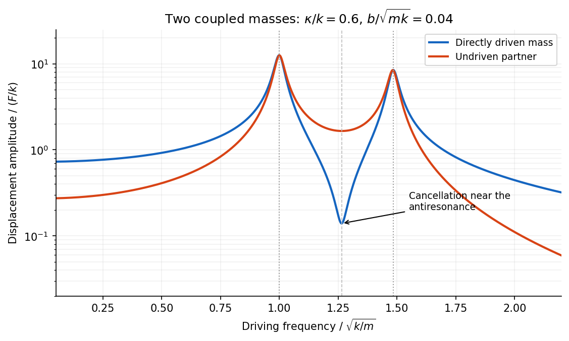
The displacement of a particular mass adds contributions from both normal modes. They can cancel at an antiresonance. For $F_2=0$ and no damping, $x_1$ vanishes at ${\Omega }^2=(k+\kappa )/m$, while the partner still moves. This differs from the two nearby resonances, where a mode responds strongly; a small measured response need not mean that no motion or stored energy exists elsewhere.

A Newtonian fluid exerts viscous shear stress proportional to the rate of strain. For an incompressible fluid of constant dynamic viscosity $\eta$,The local momentum balance is the Navier-Stokes equation:The left side is density times material acceleration. A steady velocity field can still have convective acceleration when a moving parcel changes speed or direction; setting $\partial \mathbf{u}/\partial t=0$ does not eliminate it.

The Reynolds number $\mathrm{Re}=\rho UL/\eta$ compares inertia with viscous effects. At low Reynolds number, the fluid's own inertia can often be neglected, giving Stokes flow. This does not say that every immersed body has zero acceleration: its mass and the net pressure, viscous and body forces still enter its own equation of motion.

For a small rigid sphere moving through a slowly varying viscous background, Stokes drag is $-6\pi \eta a(\mathbf{v}-\mathbf{u})$. In still fluid, a simple settling model includes weight, buoyancy and drag:Ignoring fluid added mass and unsteady history forces, this gives relaxation time $m/(6\pi \eta a)$ and terminal velocityAt the terminal velocity the net force and acceleration vanish, while viscous drag and gravity remain individually nonzero. The dissipated power $6\pi \eta a{v}_t^2$ is supplied by the loss of gravitational potential energy relative to buoyant support. The creeping-flow and quasisteady-drag assumptions must be checked before applying this expression at large speed or immediately after a rapid start.

For two bodies interacting through a potential energy that depends only on their separation, introduce the centre of mass coordinate and the two-particle relative coordinate:Their kinetic energy separates exactly:The centre of mass moves uniformly if there is no external force, while the internal two-body problem reduces to one effective particle of reduced mass $\mu$:The original trajectories follow from ${\mathbf{r}}_1=\mathbf{R}+(m_2/M)\mathbf{r}$ and ${\mathbf{r}}_2=\mathbf{R}-(m_1/M)\mathbf{r}$.

For Newtonian gravity, $U=-G{m}_1{m}_2/r$, so the relative acceleration is $\ddot{\mathbf{r}}=-GM\mathbf{r}/r^3$. Conserved relative angular momentum and energy then give the usual conic sections. For a bound orbit of relative semimajor axis $a$,The two bodies share this orbital period and orbit their common centre of mass with semimajor axes in inverse proportion to their masses. If $m_2\gg m_1$, then $\mu \simeq m_1$, recovering the fixed-heavy-centre approximation. Using $M$ as the internal inertial mass would confuse centre-of-mass translation with relative motion.

Elasticity describes recoverable deformation. For small displacements $\mathbf{u}(\mathbf{x})$, the infinitesimal strain tensor is the symmetric part of the displacement gradient,Its diagonal entries describe extension, while its off-diagonal entries describe shear. The engineering shear strain is ${\gamma }_{xy}=2{ϵ}_{xy}$; the antisymmetric part of the displacement gradient is a small rigid rotation, not elastic strain.

The stress tensor specifies the force per unit area on each oriented plane: $\mathbf{t}(\hat{\mathbf{n}})=\mathbf{\sigma }\hat{\mathbf{n}}$. Positive normal stress is tensile in the convention used here; tangential traction gives shear stress. In the absence of internal couples, angular-momentum balance makes the stress tensor symmetric. Force balance gives $\nabla \cdot \mathbf{\sigma }+\mathbf{f}=0$ in static equilibrium, where $\mathbf{f}$ is body force per unit volume.

Linear elasticity relates stress and strain. A homogeneous isotropic solid needs two independent elastic constants:Here $G$ is the shear modulus and $\lambda$ is the other Lamé parameter. For uniaxial loading, Young's modulus is $E={\sigma }_{xx}/{ϵ}_{xx}$, with lateral contraction described by Poisson's ratio $\nu =-{ϵ}_{yy}/{ϵ}_{xx}$. The bulk modulus is $K=-p/(\Delta V/V)$ for a small hydrostatic compression. The relations between these constants areStable isotropic elastic strain energy density requires $G>0$ and $K>0$, implying $-1<\nu <1/2$. The incompressible limit is approached as $\nu \to 1/2$. Anisotropic crystals generally need more constants; the isotropic relations should not be imposed on arbitrary directions in such a crystal.

The elastic energy density is $w=\mathbf{\sigma }:\mathbf{ϵ}/2$. In the isotropic linear model this becomes $\lambda (\mathrm{tr}\mathbf{ϵ}{)}^2/2+G\mathbf{ϵ}:\mathbf{ϵ}$. The quadratic form explains why reversible loading stores energy and unloading can return it, unlike plastic deformation or a dissipative hysteresis cycle.

For a slender beam described by the Euler-Bernoulli beam equation, plane sections approximately remain plane. A fibre a distance $y$ from the neutral axis has axial strain $-y\kappa$, where $\kappa$ is curvature, and stress $-Ey\kappa$. Integrating its moment about the neutral axis gives, with consistent signs,$I_A$ is a second moment of area, with units of length to the fourth power; it is not a mass moment of inertia. For a rectangular section of width $b$ and thickness $h$, $I_A=b{h}^3/12$, explaining the strong dependence of bending stiffness on thickness. For small transverse deflection $w(x)$, curvature is approximately $w^{\prime \prime }$, and the Euler-Bernoulli beam equation is $E{I}_A{w}^{\prime \prime \prime \prime }=q(x)$ with a suitable load-sign convention. A cantilever of length $\ell$ under end load $F$ has tip deflection $F{\ell }^3/(3E{I}_A)$ and largest bending stress of magnitude $F\ell c/I_A$, where $c$ is the furthest distance from the neutral axis.

In torsion of a solid circular shaft, a cross-section rotated by angle $\theta (x)$ has shear strain $r{\theta }^{\prime }(x)$. ThereforeHere $J$ is the polar second moment of area. A uniform shaft of length $\ell$ under constant torque twists by $\mathcal{T}\ell /(GJ)$, and its largest shear stress is $\mathcal{T}a/J$. Noncircular sections can warp, so replacing their torsional stiffness by $G$ times their polar area moment is not generally valid. Both bending and torsion formulas presume small, elastic deformations; exceeding the elastic limit can produce permanent deformation or fracture.