Original solutions to the released 2016 paper. [ref]
https://www.whatdotheyknow.com/request/natural_science_tripos_physics_e_2/response/2340776/attach/2/FOI%202023%20399%20Zahid%20materials.pdf?cookie_passthrough=1#page=186. Original public PDF, physical pages 186–194; question pages 187–194
Take a long strip along , occupying in , with uniform surface current . Above the strip's centre, the contributions odd in cancel, while the Biot-Savart law gives the magnetic field of a uniformly conducting stripThe field reverses below the strip. Its field lines wrap around the longitudinal current: nearly parallel to the faces near the centre, then curving round the edges and approaching circles at large distances. The sketch is an original field integration; the conductor thickness is idealized as negligible.
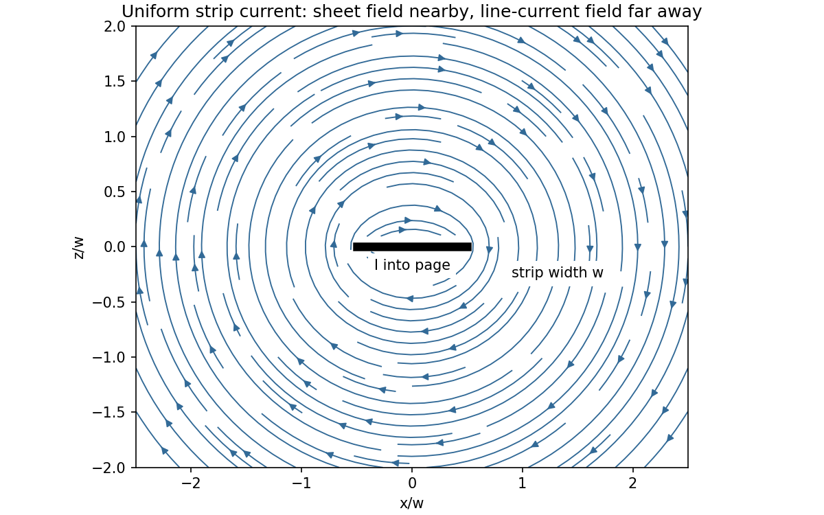
Original magnetic field-line integration for a uniformly current-carrying thin strip
. Details. At distance , the strip is indistinguishable to leading order from a straight line current. Ampère's law on a large circular contour gives , directed tangentially around the strip's longitudinal axis by the right-hand rule. On the perpendicular centreline this also follows by expanding .
At perpendicular distance from the middle of a face, but outside the conductor, the strip approximates an infinite current sheet. The tangential field jump is and symmetry gives equal opposite fields on the two sides. Hence on either side. The centreline integral gives the same limit as . Uniform current across the width and distance from the strip edges are implicit in this sheet approximation; a nonuniform surface current would require its local value instead.
Let be the initial plan area and take compression normal to the sheet. Smooth plates exert no lateral traction, so the uniaxial stress is and the two lateral strains are . To first order in strain,This area expansion under uniaxial compression is the increase of the sheet's plan area, equivalently the area of either broad face. Counting the sum of both broad faces would give twice this change; edge area would require thickness information. The cancellation of is a small-strain linear-elastic result, not a statement that arbitrarily large compressions need no geometry data.
Use a cold, unmagnetized, collisionless plasma with a sharp interface, and take the incident medium to be vacuum. Its relative permittivity is , so at the stated frequencies . Conservation of tangential wavenumber givesFor oblique total reflection at an unmagnetized plasma, require , or . Thus total reflection occurs for measured from the normal, up to grazing incidence. At the ideal critical angle the transmitted normal energy flux also vanishes, so the lossless reflectance reaches unity there. Collisions or an imposed magnetic field change this simple criterion. The constitutive response used here follows the electron-motion derivation in the cited university notes.[ref]
Oscillations and Waves by Richard Fitzpatrick. Section 9.7, equations 9.27–9.30, unmagnetized-plasma dispersion and refractive index
To obtain the maximum work from two finite heat reservoirs, operate a reversible heat engine between the bodies until their temperatures coincide. Include the work store in the isolated total system: no heat enters from outside, while the bodies can transfer energy to that store. With the stated constant heat capacities, reversibility requiresNumerically, . The decrease of the bodies' internal energy isDirect thermal equilibration without an engine would instead reach the arithmetic heat-capacity-weighted temperature and deliver no work. entropy production can only raise the final common temperature above the value for zero entropy production and reduce extractable work.
A stationary person relative to the rim has centripetal acceleration . If is a signed walking speed relative to the rim, the inertial tangential speed is , so the inward normal reaction satisfiesConsequently the support force per mass, and hence apparent weight, is for and zero for . In the latter case the walker has zero inertial speed and needs no centripetal support; ordinary weight-bearing contact cannot be assumed to persist without a restraint. For artificial gravity in a rotating ring, the centrifugal force and the Coriolis force alone are insufficient: the walker also has relative-path centripetal acceleration . Omitting it would give the wrong apparent weights at these large walking speeds.
The method of images replaces induced charges or currents on a boundary by fictitious sources outside the physical region, chosen to satisfy that boundary's conditions. For example, a point charge a height above a grounded conducting plane has an image at the reflected point. The sum has zero potential on the plane, and the electrostatic uniqueness theorem identifies it with the physical solution in the upper half-space. Images do not describe a second physical charge below the metal.
For the superconducting plane, use the different boundary condition at its surface: magnetic flux cannot enter the ideal bulk. Choose the real ring moment , where , at . Its image has moment at . This superconducting plane image dipole makes the normal fields cancel at , while their tangential fields add. The image is a computational continuation; the physical field inside the plane is zero. The original sketch shows the dipole-scale field, appropriate to ; the fine field close to the ring wire is outside that approximation.
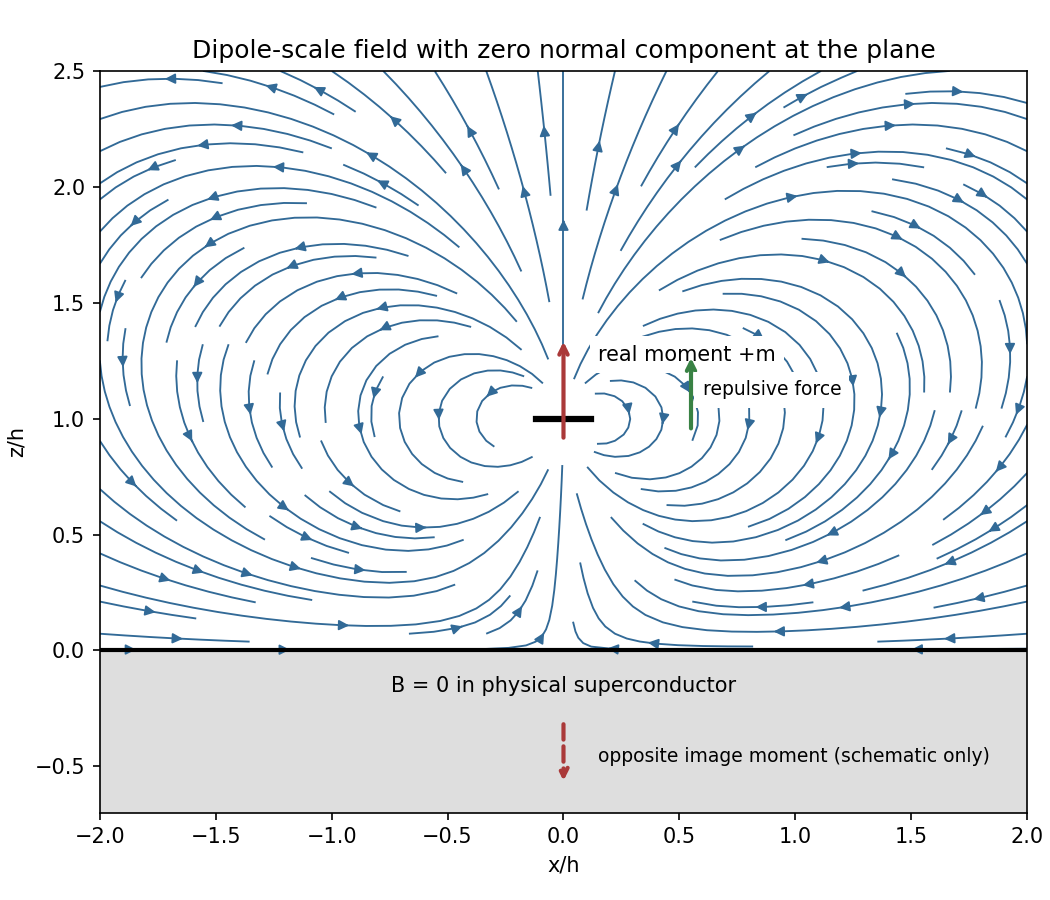
Original dipole-scale field above a flux-excluding plane, with the opposite image moment shown schematically
. Details. In the vacuum region the magnetic scalar potential isAt the surface , it reduces to . Its tangential derivative therefore givesBoth and vanish there; the sign is inward radially for the chosen positive moment. The expression is the leading dipole result, not an exact finite-ring formula at arbitrary .
For the force, calculate the external image field on the axis near the real dipole:Differentiate this field with the image location held fixed, then evaluate at . The dipole levitation force above a superconducting plane isdirected upward. Differentiating a substituted separation while moving both dipoles in the force derivative would incorrectly double the result.
To levitate ring mass , balance this force against :A light, thin wire and the smallest practical gap reduce current. At fixed gap and wire cross-section , gives , favouring a larger ring until the dipole-limit constraint on matters. There is no unique least current without geometric and material constraints. As a geometrically consistent order-of-magnitude example, take , , wire radius and an assumed metallic-scale density . Then and . The large value reflects the weak force in the stipulated far-field geometry. Uniformly shrinking this geometrical example reduces current as size to the power , but increases required electric current density; arbitrarily thin wire is therefore not a free optimization.
This balance estimate is not a verified superconducting design. The actual wire must carry that current without quenching, its self-field counts toward the limit, the plane must remain in its assumed flux-excluding state, and leads or supports add load. Transport critical-current measurements specify temperature, applied field and the voltage criterion rather than a material-independent limiting current.[ref]
Standard Reference Materials: Critical current measurements on an NbTi superconducting wire standard reference material by A. F. Clark and others. NBS SP 260-91, Section 7 and Table 3, field/temperature-dependent critical-current specification
Faraday's law for the moving loop is , equivalently for its moving circuit. Lenz's law fixes its orientation: the induced current opposes the change in linked magnetic flux. The minus sign represents this opposition, not opposition to the existing field in every phase of motion.
Unroll the small loop's motion locally into translation to the right at speed , where is the radius marked in the source figure. Take the imposed field into the page. On entry the linked into-page flux increases, so the current is counterclockwise. The leading vertical side carries current upward and feels a leftward magnetic force . The in-field parts of the horizontal sides feel equal opposite vertical forces; the trailing side is outside the field. On exit the current is clockwise. The trailing vertical side is now the one in the field and again carries upward current, producing leftward drag; the horizontal forces reverse and still cancel. When the entire loop is within the uniform region, its flux is constant, so and every side force is zero under the stated negligible-self-inductance approximation.
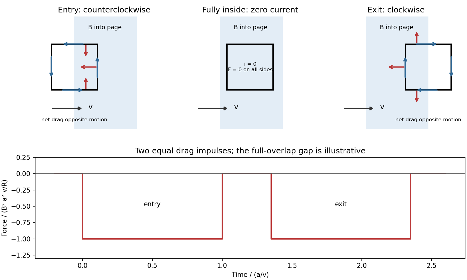
For a loop crossing a magnetic field boundary, overlap changes at rate , henceFor approximately constant speed this gives two negative rectangular force pulses of duration , separated by a short zero-force interval while the loop is fully inside. Their time integral isThe quoted impulse is its magnitude; this impulse of magnetic braking opposes the motion. In fact its independence of speed remains exact within this locally translational sharp-boundary model even if speed changes: each crossing contributes over distance .
Write the system's moment of inertia as . Since , the local energy balance during overlap isThus rotational energy lost is exactly resistive heat in this model. At nearly constant , each pass givesFor a finite speed reduction the exact relation is the integral of , rather than initial speed times impulse; the equality of work and heating still holds. Fringing fields, loop curvature and finite self-inductance smooth the ideal pulses. A practical user control is to vary the electromagnet current, hence : braking scales as .
Use peak phasors with time dependence , real positive electrical conductivity , and absolute permeability . Ampère-Maxwell equation and Faraday equations giveso . The sign of the imaginary term follows from the stated time convention. For a transverse plane wave in a homogeneous conductor,In the good-conductor limit, choose the root that decays into :The electric phasor and physical field are consequently and , as required. Tangential boundary matching sets ; it need not equal the incident amplitude.
Faraday's law fixes the magnetic field, including its phase:For real and , this means , with other components zero. The time-averaged Poynting vector isThe energy entering a thin slab exceeds that leaving it by per unit volume, givingDirectly, and at each time. Therefore is exactly this loss. The factors one half use peak rather than root mean square phasors; amplitude decays over , while intensity decays over .
For a cold collisionless unmagnetized plasma, electron inertia gives and real . Above the plasma frequency the wave propagates without this resistive attenuation. Below it, a semi-infinite plasma supports an evanescent field with electric and magnetic components in quadrature and zero mean inward energy flux: the incident energy is reflected, not absorbed as Joule heating. electron kinetic energy is reversibly stored, so the nondispersive dielectric field-energy formula alone is incomplete. Collisions introduce a real dissipative electrical conductivity and can produce absorption.[ref]
Oscillations and Waves by Richard Fitzpatrick. Section 9.7, equations 9.36–9.53, evanescence, phase quadrature and unit reflectance
For a linear nondispersive medium with real absolute permittivity and permeability , instantaneous field energy density and energy flux arewith local balance . energy stored locally and energy passing through a surface are distinct: integrating the balance relates their rates and the power given to charges.
Between the coaxial conductors, cylindrical Gauss and Ampère laws giveThe inner line charge is , so the capacitance per length is . Integrating magnetic energy over the annulus gives , hence . ThusThese are per-length parameters for ideal conductors, excluding internal magnetic penetration.
Now let the voltage and current amplitudes be and multiply both transverse fields by . Their divergences vanish in the annular dielectric. The two nontrivial curl equations reduce toConsequently both and are required for a forward wave. Arbitrary independent static and cannot acquire the same forward-wave factor and still satisfy Maxwell's equations. This TEM travelling-wave voltage-current relation and the dispersion constraint identify the transverse electromagnetic mode and its speed .
For the travelling wave, . Integrating over the dielectric annulus yieldsThis is the familiar circuit power, carried here through the dielectric rather than through the ideal metal. In root mean square notation it is for the forward lossless wave; the corresponding static fields give without a time-average factor. The average line energy is , whose product with wave speed agrees with the power.
Finite conductor resistance requires a small longitudinal electric field to drive current. Its cross product with the azimuthal magnetic field produces a radial Poynting component into each conductor: inward radially at the inner conductor and outward radially into the outer conductor. This Poynting flux into lossy coaxial conductors explains why forward power decreases along the cable as energy becomes heat in the metal. The mode is then only approximately TEM; strictly zero longitudinal electric field would be inconsistent with resistive current.
For a central potential, angular momentum is conserved and the motion lies in a plane. With , radial energy conservation becomesAllowed radii have ; equality gives radial turning points. A well with two finite turning points gives regular radially bound motion. Access to arbitrarily large radii gives an unbound branch, while access to the origin can lead to collision in a singular potential. Stationary points are circular-orbit candidates; a strict local minimum gives radial stability. For a potential tending to zero at infinity, energy relative to that asymptote is useful, but a singular inner potential and centrifugal barrier must still be examined.
Integrating the angular-momentum relation with the origin of angle at givesFor at , the effective potential is . It is exactly the Kepler effective potential with , provided that expression is real. Equal radial energy and initial radial phase therefore give identical , although the angular motion differs. Writing for the Kepler angle, . With matched periapsis origins,Here and the eccentricity is fixed by radial energy. For , and successive periapses are separated by , so there is retrograde apsidal motion relative to a closed Kepler ellipse. The radial equivalence is the relevant content of the Newton's theorem of revolving orbits.
For the pure inverse-cube central force set . The free-particle reference orbit at is a straight line, , not a finite- conic with its old held fixed. To cover attractive as well as repulsive cases completely, putwhere primes denote angle derivatives and . The inverse-cube central orbit classification gives the following physically positive-radius branches.
For , write with , so . These are scattering orbits with positive energy and an inner turning radius ; the angular interval between the two infinite-radius ends is . Repulsion () gives an interval smaller than ; weak attraction () gives a larger interval and can cause winding. The limit is the straight line.
For , . If , reciprocal-linear spirals connect an infinite-radius end to collision at infinite accumulated angle. If and , every radius admits a circular solution at zero energy: attraction exactly balances centrifugal acceleration. Each is a marginal circular orbit under an inverse-cube force, with no radial restoring force.
For , put and . Up to angle shifts and reversal, the three energy classes arewith positive-radius domains understood. The negative-energy branch is radially bounded but reaches the singular centre on either side of its outer turning point; it is not a regular closed orbit. Collision requires additional physics to continue through . Zero angular momentum gives radial trajectories and is excluded from the angular parametrization above.
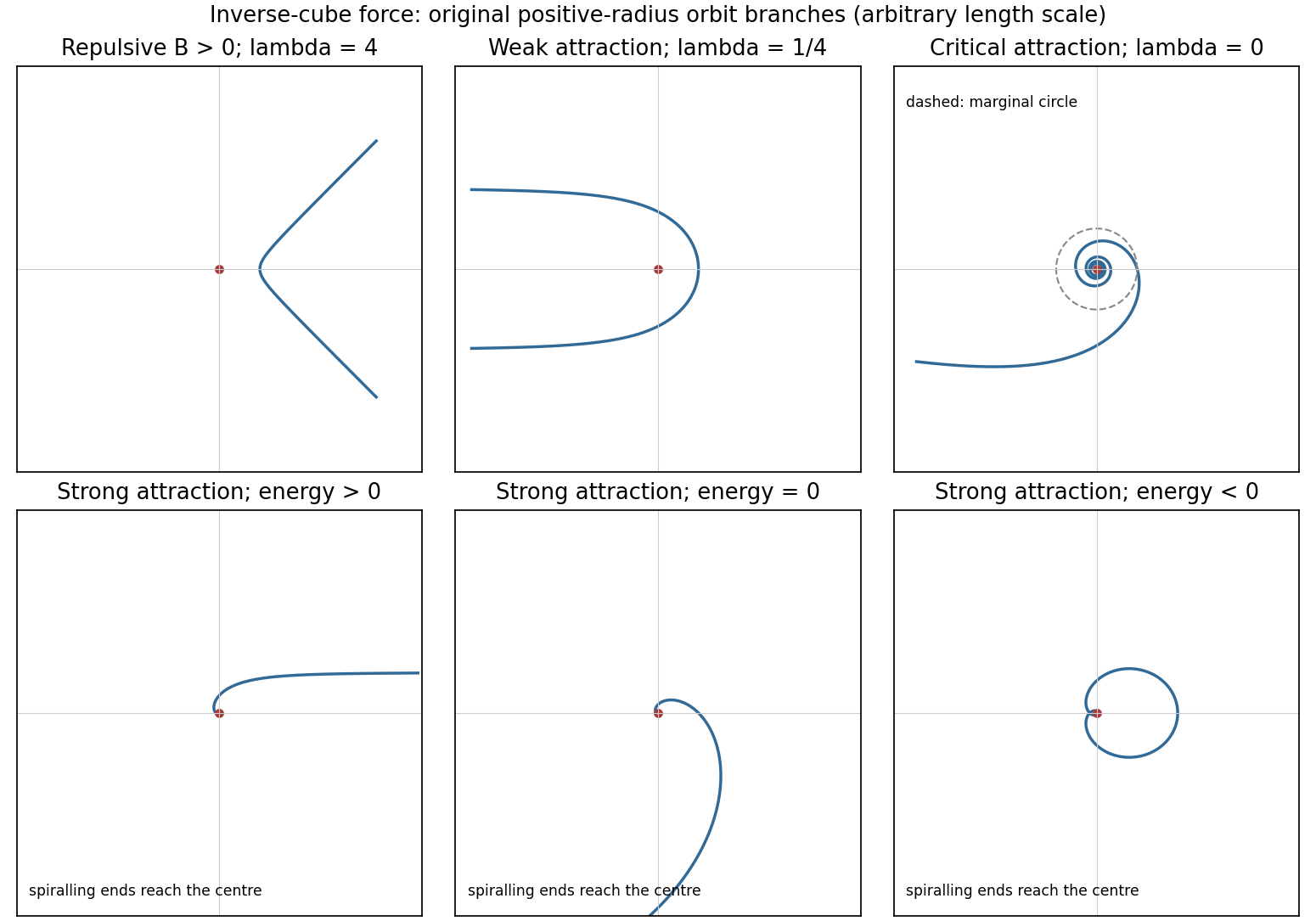
Original representative inverse-cube orbit branches, with force sign and critical attraction distinguished
. Details. For a body-fixed mass element at position relative to the fixed tip, . ThereforeThe inertia tensor is real symmetric. Its orthogonal eigenvectors define principal axes and its eigenvalues are principal moments of inertia. angular momentum is parallel to angular velocity when rotation is along a principal axis, but generally not for arbitrary rotation.
Write and . Axial symmetry gives . Since , the vector triple-product identity gives . HenceDifferentiate in the inertial frame, using constant and . The gravitational torque about the fixed tip is , yielding the symmetry-axis equation of a heavy symmetric top:The tip reaction exerts no moment about that tip.
For steady precession, . At azimuth zero, put and . Then , , and the component gives . For a nonvertical axis this becomesReal steady branches require a nonnegative discriminant. In particular, for a top pointing above the horizontal there is a spin threshold for these fixed-angle solutions. At use the quadratic's linear limit , rather than dividing by zero. For a vertical axis, azimuth does not describe a physical conical motion and the division by is inappropriate.
For rapid positive spin with , the slow and fast steady precession roots areThe approximation assumes a nonsingular fixed inclination. For , the quadratic instead gives or . The zero branch has a stationary symmetry axis and pure axial spin. On the other branch angular momentum is constant and parallel or antiparallel to the chosen axis; and . This is torque-free precession in space, not the different rate at which transverse components rotate in body coordinates.
Take as signed distance from the neutral axis within the beam cross-section. Bending into a large radius changes the length of a fibre proportionally to , so linear elasticity gives , up to the curvature sign convention. The moment magnitude isHere is the second moment of area about the neutral axis, with units of length to the fourth power, not the mass moment of inertia. A homogeneous cross-section has its neutral axis through the centroid under pure bending.
For the straight pin-ended beam, the compressive dead load produces bending moment at transverse offset . In the small-slope approximation, curvature is with the corresponding sign convention, givingThe stated endpoints fix positions rather than slopes: this interpretation is consistent with the illustrated end forces and the later sinusoidal unstressed shape. Truly clamped endpoints would have a different threshold. A nonzero solution requires . Thus the first Euler load is . Below it the perfect straight state is stable, at it the first mode is marginal in linear theory, and above it the straight state is unstable. The linear equation selects thresholds but cannot set the amplitude or describe a finite postbuckled equilibrium.
For the initially curved compressed beam, elastic stress responds to the change from its stress-free curvature. With , the moment is , so force balance givesPut and seek the branch continuously connected to the unloaded shape. Since , substitute to obtain , orAway from eigenvalues, the homogeneous solution vanishes under the two end conditions, so this particular solution is the unique linear equilibrium. For and , the maximum additional displacement is and maximum total displacement is , both at midspan.
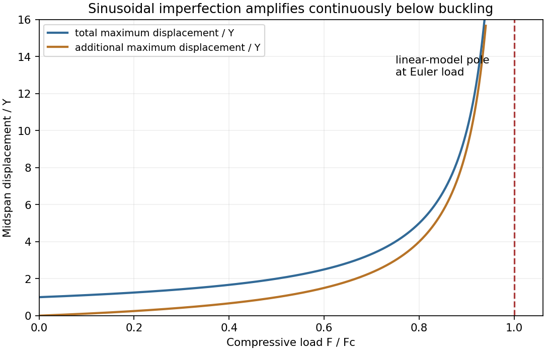
This sinusoidal imperfection amplification of a column produces deflection at every positive load and strong amplification near . The apparent divergence signals loss of the small-slope model before infinite displacement; nonlinear geometry is needed there. The formal continuation above the first threshold is not a stable physical loading branch. Both total and additional displacement are distinguished in the graph.
irrotational flow has , so locally ; the simply connected fluid domain here permits a globally single-valued velocity potential. Incompressibility gives , hence . In a multiply connected domain, zero local vorticity alone would not rule out circulation and a multivalued potential.
Take so the disturbance decays at depth. Differentiating the given candidate potential yieldsThe and second derivatives of cancel in the Laplacian. At , , so the linearized kinematic free-surface condition holds. This uses ; advection of the displaced surface is higher order.
Since , the local squared speed is . The depth integral is thereforeIt is independent of horizontal position; no further spatial average is needed for this kinetic energy. Replacing the upper boundary by zero changes it only beyond quadratic order in amplitude.
Relative to the flat surface, the gravitational energy at each horizontal position changes by . Averaging over one wavelength givesThe energy of a deep-water standing gravity wave, averaged over wavelength, is and must be constant for a free inviscid standing wave, which requires equal coefficients of the complementary squared sine and cosine:As an independent check, the linearized dynamic boundary condition at gives exactly . Infinite depth, negligible surface tension and no dissipative forcing are part of this gravity-wave model.
The Boltzmann entropy isThe thermodynamic definition of temperature givesHolding the other system parameters fixed, , so its heat capacity is . The constants and set an additive reference for entropy; neither affects this derivative or the resulting heat capacity.
For a lossless transmission line with characteristic impedance and resistive termination , the voltage reflection coefficient isThe reflected pulse is inverted and has half the incident voltage, so . Substituting the termination givesThe echo delay is a round trip from the observation point to the termination and back, not a one-way travel time. Thus the propagation speed isFor a homogeneous, nonmagnetic coaxial cable dielectric, , giving . More generally the measured speed fixes ; identifying this with relative permittivity assumes and negligible dispersion or attenuation of the pulse.
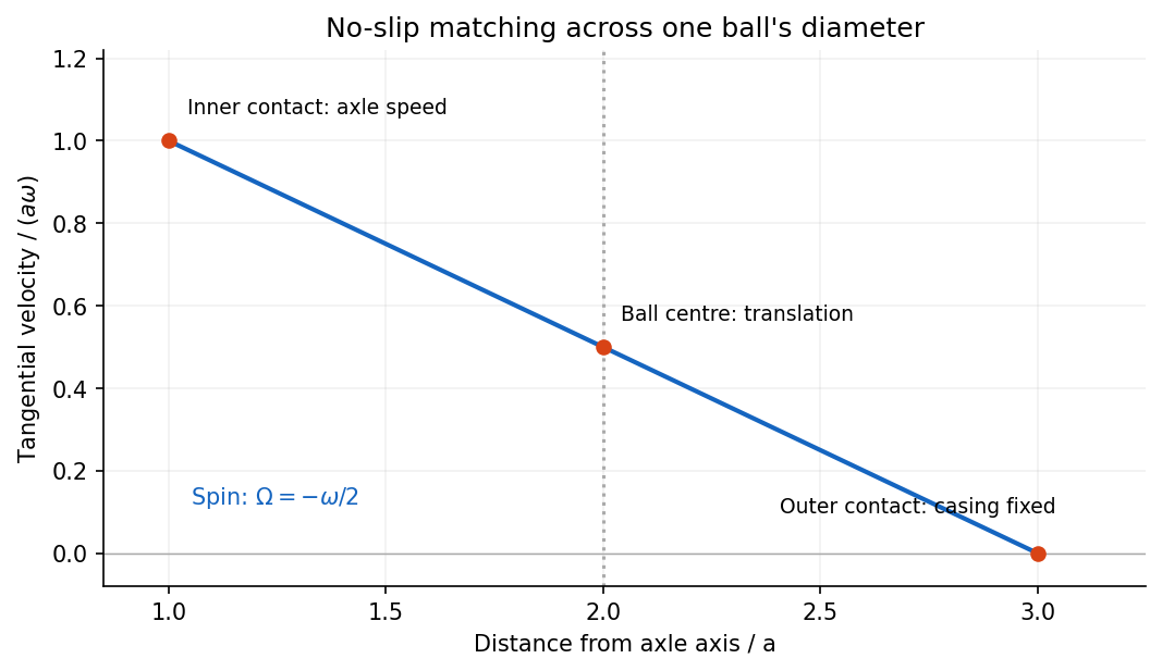
Separate a ball's orbital motion from its spin. For a rolling ball between concentric races, the ball centre lies from the axle axis. Let its tangential centre velocity be in the direction of axle motion and let its signed spin angular velocity be , positive in the same sense as . Rolling without slipping at the moving inner contact and stationary outer contact requiresHenceThe spin is opposite to the axle's rotation, while the centre orbits in the same sense. The total angular momentum about the axle is the sum of its orbital angular momentum and its angular momentum about the centre of mass:For a uniform solid spherical ball, , soThe solid-ball assumption supplies the usual moment of inertia; the preceding expression in terms of also states the answer for a different internal mass distribution.
In the thin-gap Couette flow approximation, the tangential velocity varies linearly through the gap. At radius , its difference between the two discs is , so a Newtonian fluid exerts shear stressAn annulus has area , and its tangential force acts at lever arm . Integrating its torque givesThe driving torque is in the direction of rotation; the liquid's resisting torque has the opposite sign. This parallel-disc viscometer result assumes laminar shear with no slip, negligible edge effects and negligible secondary circulation. Its fourth-power radius dependence comes from the combined radial dependence of speed, annular area and lever arm.
At fixed temperature, equilibrium blackbody radiation has fixed energy density , with radiation pressure . Doubling the volume therefore doubles its internal energy, so . The work done by the radiation isThe first law of thermodynamics, with positive work done by the radiation, givesThus is absorbed from the walls. The walls must replace the energy used to do work as well as supply the extra stored energy; using only would omit that work. This is a reversible isothermal expansion of a photon gas, not an adiabatic expansion.
An electric dipole consists of equal and opposite electric charges separated by a displacement . Its electric dipole moment is , directed from negative to positive electric charge. At distances large compared with the separation, its leading electric potential and electric field areThere is no monopole term because the net electric charge is zero. The axial electric field points along with magnitude , while the equatorial electric field points oppositely with half that magnitude.
A uniform applied electric field exerts zero net force on an ideal fixed electric dipole, but it exerts torque . Its orientation-dependent potential energy is , so alignment with the electric field is stable. A nonuniform applied electric field can also exert a net force, for a fixed permanent electric dipole moment.
A permanent electric dipole moment exists without an applied electric field. An induced electric dipole moment instead develops in response to the local electric field; in an isotropic linear model . Creating that induced moment requires accounting for the work of polarization, so its mechanical potential energy in a specified applied electric field is , rather than . In matter, the dipole moment per unit volume is the polarization density .
Mutual inductance expresses how a changing electric current in one circuit induces an electromotive force in another. Choose winding orientations and define their linked magnetic fluxes byFor a reciprocal linear magnetic system, the same appears in both expressions. Faraday's law of induction gives when the secondary electric current does not itself change. The sign depends on winding orientation and is consistent with Lenz's law.
The stored magnetic energy isIts nonnegativity for arbitrary electric currents requires . Strong coupling makes approach ; flux leakage makes it smaller.
An ideal electrical transformer has two windings linked by the same time-varying core magnetic flux. The induced winding voltages are proportional to their turn counts. For appropriately chosen terminal polarities,The electric current convention in the power relation takes primary power into the device and secondary power out to the load. Consequently a load electrical impedance appears at the primary as . A larger secondary voltage therefore comes with a smaller available secondary electric current, rather than extra energy.
A steady direct electric current produces no sustained transformer action after its switching transient. Practical departures from the ideal include winding electrical resistance, leakage magnetic flux, finite magnetizing electric current, core saturation, eddy currents and magnetic hysteresis losses.
Free charge is charge assigned to externally supplied or mobile carriers in a macroscopic description. Bound charge describes the net charge associated with a material's polarization density . Its bulk and surface densities arewhere the normal points out of the polarized material. Uniform bulk polarization density has no bulk bound charge, but it can still have surface bound charge.
The electric field is sourced by the total electric charge. Introducing the electric displacement field separates the free source in the macroscopic field equation:This does not mean that bound charges are physically absent from : they are represented through . In a linear isotropic dielectric, and , with .
Across a stationary ordinary dielectric interface, electrostatics gives continuity of tangential electric field, while a free sheet charge givesThe normal electric field need not be continuous. For a fully filled parallel-plate capacitor at fixed free plate charge, polarization reduces the internal electric field by and increases capacitance by the same factor. If a battery instead holds the voltage fixed, extra free plate charge flows from the battery; the constraint must be stated before comparing stored energies.[ref]
The Feynman Lectures on Physics, Volume II by Richard Feynman and others. Chapter 10, §§10–1 to 10–4: dielectric capacitor, polarization charge and the field equations
A permanent magnet retains a substantial magnetization without an applied coil electric current. In a ferromagnetic material this reflects microscopic magnetic moments, magnetic domains and their resistance to rearrangement. The history-dependent relation between applied field and magnetization gives magnetic hysteresis, remanence and coercivity. A soft core used in an electromagnet or electrical transformer is chosen for easy magnetization and small hysteretic loss; a permanent-magnet material must resist demagnetization.[ref]
The Feynman Lectures on Physics, Volume II by Richard Feynman and others. Chapter 36, especially §36–3 and Figures 36–8 to 36–9: magnetization curves, remanence and hysteresis loss
The macroscopic fields obeyin magnetostatics. The magnetization can be represented by equivalent bound currents,Thus both permanent magnetic matter and free coil electric currents generate a magnetic field. Its magnetic field lines form continuous loops; apparent north and south poles are not isolated magnetic charges.
In a long ideal solenoid, . A linear core would give , until saturation or other nonlinear effects invalidate a constant magnetic permeability. In a finite magnetic circuit, air gaps and demagnetizing fields affect the field strongly: because the gap has low magnetic permeability, it often needs most of the available magnetomotive force. A permanent magnet can have a nonzero internal even when , because its boundaries create a demagnetizing field. Hence setting merely because there is no free coil electric current is generally incorrect.
An electrostatic field calculation begins by specifying the charge information, material response and boundary conditions. In vacuum, prescribed volume and surface electric charge densities can be superposed directly using Coulomb's law. For a volume distribution,Differentiating this electric potential gives the electric field. This is useful for known source distributions, but in the presence of conductors the induced surface electric charge is usually an unknown rather than an independently specified input.
Gauss's law is especially effective when symmetry fixes the direction and magnitude of the electric field on a suitable closed surface. A spherical charge distribution gives a radial field, an infinitely long uniform line gives a cylindrical field, and a uniform infinite sheet gives a planar field. In an arbitrary geometry, the flux law remains true but does not alone determine the pointwise electric field. A multipole expansion is another useful approximation: far from a localized charge distribution, successive monopole, dipole and higher terms separate the effects of total charge and its spatial structure.
For a boundary-value formulation, use the electrostatic equationsThey imply Poisson equation , or Laplace equation where . A conductor in electrostatic equilibrium is an equipotential with zero internal electric field. Its exterior normal electric field fixes the surface electric charge through . One must specify whether each conductor is grounded, maintained at a prescribed voltage, or isolated with prescribed total electric charge.
Uniqueness of Poisson equation justifies methods that construct a convenient candidate solution. With fixed boundary electric potential and suitable behaviour at infinity, a solution satisfying the field equation is the solution. With normal-derivative boundary conditions, the source and flux must be compatible, and the electric potential is determined only up to an additive constant.
For example, a point charge a distance above a grounded infinite plane has the same upper-half-space electric potential as and a mirrored image charge below it. Their potentials cancel on the plane. The image is a mathematical source in the excluded region, not a second physical charge. Separation of variables similarly constructs solutions suited to rectangular, cylindrical or spherical boundaries; matching coefficients enforces the prescribed boundary data.
In dielectrics, the distinction between total and free charge is essential. In a linear isotropic material,Only where permittivity is constant may this be reduced to . At an ordinary interface, and the tangential electric field are continuous, while the jump in normal electric displacement field is the free surface charge. Applying Gauss's law to total charge with , or its displacement-field form to free charge, gives consistent descriptions; mixing their sources and permittivities does not.
A useful interface example is the image charge at a dielectric interface. If lies in medium 1, the source-side potential is represented bywhere is distance to the real charge and to its mirrored position. The other-side potential can be written , where . Continuity of and of normal fixes both coefficients. The equal-permittivity limit gives no image; the conductor limit gives .
For a sphere of radius and relative permittivity in a uniform external electric field , matching the spherical solutions gives a uniform internal electric field and an external induced electric dipole moment:This illustrates how a material boundary modifies an otherwise simple applied electric field.
For complex boundaries or spatially varying materials, finite difference methods or the finite element method solve the same boundary value problem numerically. A sound calculation checks its boundary conditions, charge or flux balance and convergence with mesh refinement. The governing equations, source classification and uniqueness argument remain the organizing principles even when an analytic formula is unavailable.
A horizontal pressure gradient force accelerates air from higher toward lower pressure. In a rotating frame the Coriolis force deflects the flow. Away from strong friction, at large spatial scales and small Rossby number, a slowly changing flow can reach geostrophic balance:where is the Coriolis parameter. The geostrophic wind runs along atmospheric isobars, with speed . Closely spaced atmospheric isobars therefore indicate stronger geostrophic wind when density and latitude are comparable. In the northern hemisphere lower pressure lies to the left of this wind, producing counterclockwise circulation around a low; the sense reverses in the southern hemisphere.
A curved flow also has centripetal acceleration. For cyclonic circular flow in the northern hemisphere, the gradient wind relation isNear the ground, friction reduces wind speed and weakens its Coriolis contribution, so air crosses atmospheric isobars toward lower pressure. The simple geostrophic formula fails near the equator, where becomes small, and where rapid changes or tight curvature make neglected acceleration important. Vertically, large-scale motion is often approximated by hydrostatic balance, .
Bernoulli's principle can relate speed changes to pressure changes along an appropriate inviscid streamline, but its simple dynamic-pressure relation is not a replacement for the rotating force balance governing a broad atmospheric pressure map.
Coupled oscillators have more than one collective pattern of motion. For two equal masses , each attached to a fixed support by a spring of stiffness and linked to each other by stiffness , small displacements obeyHere equal linear damping is included to make finite steady-state responses at resonance. The normal mode coordinates and diagonalize these equations. Their natural angular frequencies areThe symmetric normal mode leaves the coupling spring unextended; the antisymmetric normal mode stretches it and therefore has the higher frequency. With , their complex steady-state responses areThus the drive's spatial pattern matters as well as its frequency. Equal in-phase forces drive only the symmetric normal mode; opposite forces drive only the antisymmetric one; driving a single mass generally excites both. Finite damping broadens the resonance peaks and produces a phase lag. In the ideal undamped system, a resonant drive with nonzero projection onto a normal mode produces secular growth rather than a bounded resonant steady state.
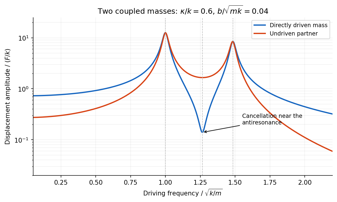
The displacement of a particular mass adds contributions from both normal modes. They can cancel at an antiresonance. For and no damping, vanishes at , while the partner still moves. This differs from the two nearby resonances, where a mode responds strongly; a small measured response need not mean that no motion or stored energy exists elsewhere.
A Newtonian fluid exerts viscous shear stress proportional to the rate of strain. For an incompressible fluid of constant dynamic viscosity ,The local momentum balance is the Navier-Stokes equation:The left side is density times material acceleration. A steady velocity field can still have convective acceleration when a moving parcel changes speed or direction; setting does not eliminate it.
The Reynolds number compares inertia with viscous effects. At low Reynolds number, the fluid's own inertia can often be neglected, giving Stokes flow. This does not say that every immersed body has zero acceleration: its mass and the net pressure, viscous and body forces still enter its own equation of motion.
For a small rigid sphere moving through a slowly varying viscous background, Stokes drag is . In still fluid, a simple settling model includes weight, buoyancy and drag:Ignoring fluid added mass and unsteady history forces, this gives relaxation time and terminal velocityAt the terminal velocity the net force and acceleration vanish, while viscous drag and gravity remain individually nonzero. The dissipated power is supplied by the loss of gravitational potential energy relative to buoyant support. The creeping-flow and quasisteady-drag assumptions must be checked before applying this expression at large speed or immediately after a rapid start.
For two bodies interacting through a potential energy that depends only on their separation, introduce the centre of mass coordinate and the two-particle relative coordinate:Their kinetic energy separates exactly:The centre of mass moves uniformly if there is no external force, while the internal two-body problem reduces to one effective particle of reduced mass :The original trajectories follow from and .
For Newtonian gravity, , so the relative acceleration is . Conserved relative angular momentum and energy then give the usual conic sections. For a bound orbit of relative semimajor axis ,The two bodies share this orbital period and orbit their common centre of mass with semimajor axes in inverse proportion to their masses. If , then , recovering the fixed-heavy-centre approximation. Using as the internal inertial mass would confuse centre-of-mass translation with relative motion.
Elasticity describes recoverable deformation. For small displacements , the infinitesimal strain tensor is the symmetric part of the displacement gradient,Its diagonal entries describe extension, while its off-diagonal entries describe shear. The engineering shear strain is ; the antisymmetric part of the displacement gradient is a small rigid rotation, not elastic strain.
The stress tensor specifies the force per unit area on each oriented plane: . Positive normal stress is tensile in the convention used here; tangential traction gives shear stress. In the absence of internal couples, angular-momentum balance makes the stress tensor symmetric. Force balance gives in static equilibrium, where is body force per unit volume.
Linear elasticity relates stress and strain. A homogeneous isotropic solid needs two independent elastic constants:Here is the shear modulus and is the other Lamé parameter. For uniaxial loading, Young's modulus is , with lateral contraction described by Poisson's ratio . The bulk modulus is for a small hydrostatic compression. The relations between these constants areStable isotropic elastic strain energy density requires and , implying . The incompressible limit is approached as . Anisotropic crystals generally need more constants; the isotropic relations should not be imposed on arbitrary directions in such a crystal.
The elastic energy density is . In the isotropic linear model this becomes . The quadratic form explains why reversible loading stores energy and unloading can return it, unlike plastic deformation or a dissipative hysteresis cycle.
For a slender beam described by the Euler-Bernoulli beam equation, plane sections approximately remain plane. A fibre a distance from the neutral axis has axial strain , where is curvature, and stress . Integrating its moment about the neutral axis gives, with consistent signs, is a second moment of area, with units of length to the fourth power; it is not a mass moment of inertia. For a rectangular section of width and thickness , , explaining the strong dependence of bending stiffness on thickness. For small transverse deflection , curvature is approximately , and the Euler-Bernoulli beam equation is with a suitable load-sign convention. A cantilever of length under end load has tip deflection and largest bending stress of magnitude , where is the furthest distance from the neutral axis.
In torsion of a solid circular shaft, a cross-section rotated by angle has shear strain . ThereforeHere is the polar second moment of area. A uniform shaft of length under constant torque twists by , and its largest shear stress is . Noncircular sections can warp, so replacing their torsional stiffness by times their polar area moment is not generally valid. Both bending and torsion formulas presume small, elastic deformations; exceeding the elastic limit can produce permanent deformation or fracture.
A Carnot cycle consists of two reversible isothermal branches joined by two reversible adiabatic branches. Let the hot isothermal expansion run from volume to , and the cold isothermal compression from to . For moles of an ideal gas, their absorbed and rejected heat magnitudes areOn a reversible ideal-gas adiabat, is constant. Applying this to the two joining branches gives . ThereforeThe result is independent of the gas's heat-capacity ratio. This derivation presumes the usual constant-heat-capacity ideal-gas model; more generally the equal entropy changes on the two isotherms give the same heat ratio without that restriction.
To establish the upper bound, suppose an engine were more efficient between these same two reservoirs. Use its output work to drive a reversed Carnot cycle, scaled so that the work magnitudes match. For fixed work , the hypothetical engine would take from the hot bath, whereas the reversed Carnot cycle would return to it. The combined device would transfer heat from the cold bath to the hot bath without any net external work. That contradicts the Clausius statement of the second law. Hence no such two-reservoir engine can exceed .
For the triangular cycle, call the three successive vertices , and measure energies in units of . For one mole of a monatomic ideal gas, , and positive work done by the gas is . The net values on the three complete branches areThus the net work is , equal to the triangle's enclosed area.
There is a small but important distinction between the net heat on a branch and its total positive heat input to a cycle. On the sloping branch put , so , with . ThenThere is a heat-flow reversal along a thermodynamic path at . The first part absorbs heat; the final part rejects it. Integrating the two signed contributions separately givesThe true total absorbed and rejected heats and thermal efficiency are thereforeFor clarity, the positive heat input on is , on it is , and on it is zero. Using just the positive net heats of the complete branches would give and ; that shortcut misses the short heat-rejection interval on .
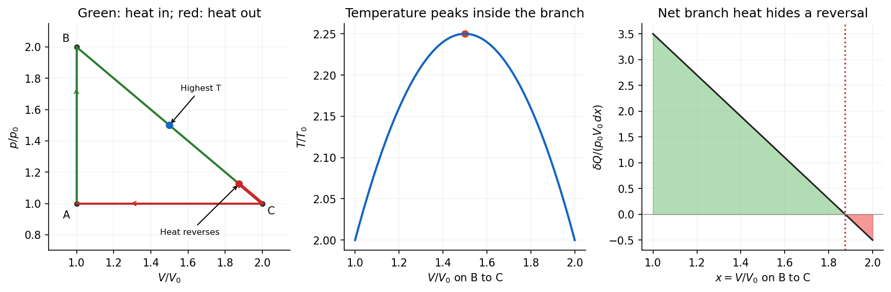
Original pressure-volume cycle with the interior temperature maximum and the late reversal of heat flow
. Details. Finally, put . The minimum temperature is at . Along ,which has its maximum at , not at either endpoint. Thus the corresponding two-reservoir Carnot efficiency isThe triangular cycle receives heat at a range of temperatures below and rejects it at temperatures above . It therefore makes less work per unit input heat than a Carnot cycle using only those extrema. The geometric path alone does not prove irreversibility: it could in principle exchange heat reversibly with a continuum of matched-temperature reservoirs, while still having this lower efficiency. Restricting it to only the two extreme-temperature reservoirs would introduce additional irreversible heat transfers.
The classical equipartition theorem assigns mean energy to each independent quadratic term in the Hamiltonian, provided the canonical distribution and its relevant boundary integrals exist. For a quadratic term , the Boltzmann distribution is proportional to , with . Integrating a total derivative givesAfter dividing by the normalization,The same argument applies to quadratic momentum terms. Other independent canonical coordinates factor out of the ratio. It is a classical statement: widely spaced quantum energy levels can freeze out a contribution at low temperature.
The confining quartic potential energy , with , is not quadratic, so the rule cannot be assigned to it. This does not invalidate the canonical Boltzmann distribution or its generalized integration-by-parts identity. Indeed,Hence equipartition for a homogeneous potential givesEquivalently, and . This is the potential contribution only; an additional standard kinetic term would contribute a further to energy and to heat capacity.
For an intact diatomic molecule, the classical degrees of freedom comprise three translational quadratic terms, two rotational quadratic terms, and two terms for its one bond-stretching vibration: one kinetic and one potential. Thus complete classical equipartition predictsThe heat capacity of a diatomic gas has lower-temperature regimes because rotational and vibrational levels are quantized. In a dilute molecular gas, the expected progression isThe rotational energy scale is normally much smaller than the vibrational scale, so these steps are separated. The high-temperature value treats the vibration as harmonic and excludes dissociation and electronic excitation; the lowest-temperature gas regime is meaningful only while the sample remains dilute and gaseous.[ref]
Statistical Physics by David Tong. §2.4, molecular rotation and vibration, and §3.4, quantum heat capacity of a diatomic gas
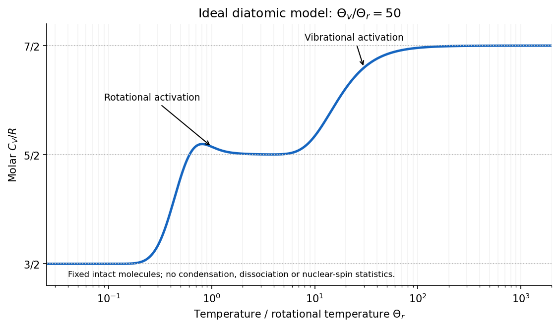
Original ideal diatomic heat-capacity model showing rotational and vibrational activation, without dissociation
. Details. The plotted example uses a quantum rigid rotor and harmonic vibration, with an illustrative ratio of characteristic temperatures. It is a model calculation, not measured data for a particular molecular species. For the vibrational part,which tends to zero on freezing out and to one when many vibrational levels are accessible. The classical equipartition theorem is recovered when the relevant level spacings are small compared with .
For the two unlabelled follow-up requests, distinguish re-equilibrating effusion from collisionless effusion. The calculations below show that escaping atoms carry mean kinetic energy , whereas a bulk atom has mean kinetic energy . If the aperture is small and interatomic collisions maintain near-equilibrium conditions, faster atoms escape preferentially, and the remaining gas relaxes toward a lower-temperature Maxwell-Boltzmann distribution. No heat supplied by the walls is available to replace the lost energy.
For a monatomic gas at fixed container volume, conservation of energy gives a quantitative check on this effusive cooling picture:Since , the temperature falls. Under these idealizations ; the gas is not left with a permanently truncated velocity tail when collisions rapidly restore equilibrium.
If interatomic collisions are absent, the individual surviving atoms do not rethermalize to a new common temperature. Their speed distribution becomes selectively depleted, generally favouring slower survivors, and their angular and spatial distribution can also develop structure determined by which trajectories reach the hole. A single lower temperature does not describe the full nonequilibrium distribution. With a direction-randomizing but energy-preserving wall model, an illustrative survival law is ; specular walls can give more detailed directional selection and even persistent nonescaping trajectories. The question supplies no wall-scattering or container-geometry model from which a unique collisionless loss law could be inferred.
For the labelled wall integrals, choose the polar axis toward the wall so that incoming atoms have , and putThe needed radial integrals are , and . They are related to the supplied integrals by rescaling the speed.
The collision flux contains an extra normal velocity : a faster atom sweeps out a longer approach cylinder per unit time. Integrating the Maxwell-Boltzmann distribution over the incoming hemisphere givesThereforeHere is the number striking unit area per unit time and is the bulk mean speed. A simple factor of one half would count the incoming hemisphere but miss the projection factor and velocity weighting.
An elastic reflection transfers normal momentum to the wall. Multiplying this impulse by the collision flux and integrating givesUsing the radial integral and yieldsThis agrees with the ideal-gas equation of state. The calculation assumes a stationary wall and elastic normal momentum reversal, appropriate to a gas in equilibrium with it.
The energy average must be taken over the atoms that actually arrive, not over the bulk population. Weighting the collision flux by givesThe wall-impact speed distribution is proportional to rather than the bulk . Faster atoms are overrepresented among arrivals. Equivalently, the mean normal kinetic energy of the arriving flux is , while each tangential component still contributes .
An equation of state relates thermodynamic variables within a material model; a phase diagram records which equilibrium phase or phases are stable under specified controls. For a pure substance at fixed temperature and pressure, stability means minimizing Gibbs free energy. Two phases coexist when their molar chemical potentials agree. The equation of state and the free-energy stability condition must therefore be used together: an algebraic relation between alone need not identify the stable branch.
A pressure-temperature phase diagram contains single-phase regions separated by phase coexistence curves. For a one-component system the Gibbs phase rule gives : a single phase has two independent controls, two-phase coexistence lies on a curve, and three phases coexist at a triple point. The liquid-gas coexistence curve ends at a liquid-gas critical point; beyond it a continuous path connects liquidlike and gaslike states without crossing a first-order coexistence boundary. A fixed point on a coexistence curve does not specify the proportions of the two phases: an additional extensive constraint, such as total volume, fixes the phase fraction.
At a first-order phase transition, first derivatives of Gibbs free energy, such as molar entropy or volume, are discontinuous. The conversion has latent heat . At a continuous transition the first derivatives match, while response functions associated with higher derivatives can be singular or discontinuous. At an ordinary liquid-gas critical endpoint, the two coexisting densities approach one another and the latent heat tends to zero; the material does not retain a sharp liquid-gas boundary above it.
The coexistence slope follows directly from equality of the two molar chemical potentials. Since , differentiating along the boundary givesThis is the exact Clapeyron equation, also commonly called the Clausius-Clapeyron relation. For vaporization, both and are positive, so the saturation pressure rises with temperature. For ordinary ice melting into liquid water, but the molar volume decreases, giving the familiar negative melting-curve slope. The sign follows from the volume change, not from a different law.
For a dilute ideal vapour with , . The ideal-vapor Clausius-Clapeyron approximation becomesIf molar latent heat is approximately constant over the interval,These approximations deteriorate close to the critical point, where liquid and gas volumes become comparable, or over a range in which latent heat changes appreciably.[ref]
Statistical Physics by David Tong. §5.1.2, coexistence slope and ideal-vapour approximation; surrounding discussion of the liquid-gas critical point and solid-liquid boundary
The ideal gas law is an equation of state for a dilute gas, but it has no liquid branch and cannot predict condensation. A simple model including repulsion and attraction is the Van der Waals molar equation,where represents excluded molar volume and represents attraction. At its critical point, , givingBelow , the homogeneous isotherm has an interval with . That would have negative isothermal compressibility and is mechanically unstable. Equilibrium liquid-gas coexistence replaces the loop by a constant-pressure segment. Equality of chemical potentials gives the Maxwell construction:The equal-area condition enforces the common tangent to the appropriate free energy; it is a stability construction rather than permission to follow the unstable loop physically. The average molar volume between and varies by changing the phase fraction.
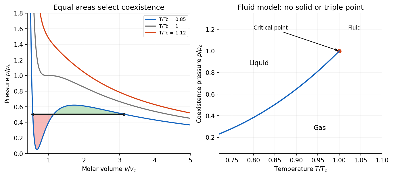


The model captures a liquid-gas critical point and qualitative coexistence, but its simple constants are not a complete quantitative description of real fluids and it has no solid phase. A full phase diagram needs additional solid free energies and can contain several crystal phases. Conversely, an experimentally determined coexistence curve and latent heat constrain equations of state through the Clapeyron equation. This is the useful connection: local thermodynamic response, global free-energy stability and the geometry of phase boundaries describe the same material at different levels.
Articles by others on the same topic
There are currently no matching articles.