Original paper: Public original PDF, physical pages 1–10; cover on page 1, blank page 2, questions on pages 3–10.
The shell theorem gives the gravity of a concentric hollow sphere as . There is no enclosed mass at the cavity boundary, whereas the entire shell has mass . ThusBoth nonzero fields point towards the centre. The field is continuous at each boundary; there is no surface mass sheet.
For drum-frequency dimensional scaling, let , where is surface mass density. The dimensions are and , so matching powers gives , and :The dimensionless normal mode constant is unchanged for the same circular shape and boundary condition. The doubled tension does not offset the doubled radius.
For a mass change in a viscously damped spring oscillator, use linear viscous damping , holding the spring constant and damping coefficient fixed. Measuring from removes the constant force. The envelope is , whereDoubling halves both and . ThereforeNeglecting damping in the frequency gives , indistinguishable at the supplied precision. The release condition sets the phase and new initial amplitude, not these envelope ratios. A different mass-dependent drag law would require its damping coefficient to be specified.
To find the magnitude uncertainty of a series RL impedance, put . Then andIf the quoted errors are independent standard uncertainties, and giveIf they denote strict bounds instead, the first-order bound is . The source does not specify their statistical interpretation, so these two error conventions should not be conflated.
The phase step between adjacent slits isFor equal amplitudes , the six unmodified contributions form a closed regular hexagon in the complex plane:Reversing one slit at an array minimum replaces slit 's contribution by its negative, so . ConsequentlyThis is independent of which slit is reversed. The result uses the far-field, narrow-slit and small-angle approximations; retaining changes the phase step only by about radians.
The breakdown-limited parallel-plate charge follows from the ideal parallel-plate capacitor relation . Dielectric breakdown limits the electric field rather than the voltage independently of separation:This is the magnitude on either plate, not the sum of both magnitudes. Edge enhancement and fringing are neglected, as in the stated parallel-plate model.
Let increase down the ramp. On a plane, static friction acts uphill. Translation and rotation giveWith , elimination yields . Static friction does no work at the stationary contact point.
For a sphere rolling in a symmetric groove, the distance from the centre to the instantaneous contact axis AB is , so . The kinetic energy and work-energy equation areHenceFor the stated angles this is . Using and a one-second descent,On the level floor the rolling radius becomes , so an energy-preserving change of rolling radius gives . ThereforeThe floor speed exceeds the groove speed because less of the same total kinetic energy is rotational. Holding the translational speed fixed at the transition would violate the stipulated energy balance with the new no-slip constraint.
Take the incident photon along , and write for the boost. In the boosted frame the initial momenta areTheir sum vanishes when , giving and . The initial photon energy there is , and total energy is .
For right-angle Compton scattering in the centre-of-momentum frame, choose the outgoing ZM photon along . The electron has the opposite momentum . Conservation of energy determines its magnitude:Thus . Inverting the velocity transformation givesConsequentlyThe electron recoils below the incident direction for our choice of photon scattering above it; the reflected configuration reverses both transverse signs. Finally,As a check, , so the final energies sum to the initial . The outgoing laboratory photon makes with .
For a fixed set of bodies in an inertial frame, total linear momentum is constant if the resultant external force vanishes. Summing Newton's second law cancels internal force pairs by Newton's third law. For an open subsystem, momentum carried across its boundary must also be included.
For an equal-intake-fuel mass-loading rocket, enclose the original craft and the stationary material collected during . Its initial momentum is . At the end, the craft has mass and the exhaust has mass . To first order,The first term is rocket thrust; the second is the momentum cost of collecting stationary matter. It vanishes in the conventional rocket equation, which therefore has no analogous fixed exhaust-speed ceiling in Newtonian mechanics. Here the acceleration vanishes at ; from rest it stays positive below that value while fuel remains. Relativistic limits are outside this model.
For constant , mass conservation gives . Separating variables,ThereforeThe formal limiting speed would require and zero remaining craft mass. A positive rocket dry mass and finite carried fuel terminate the burn earlier. Maintaining nonzero collection rate even at rest is an idealization explicitly prescribed by the problem.
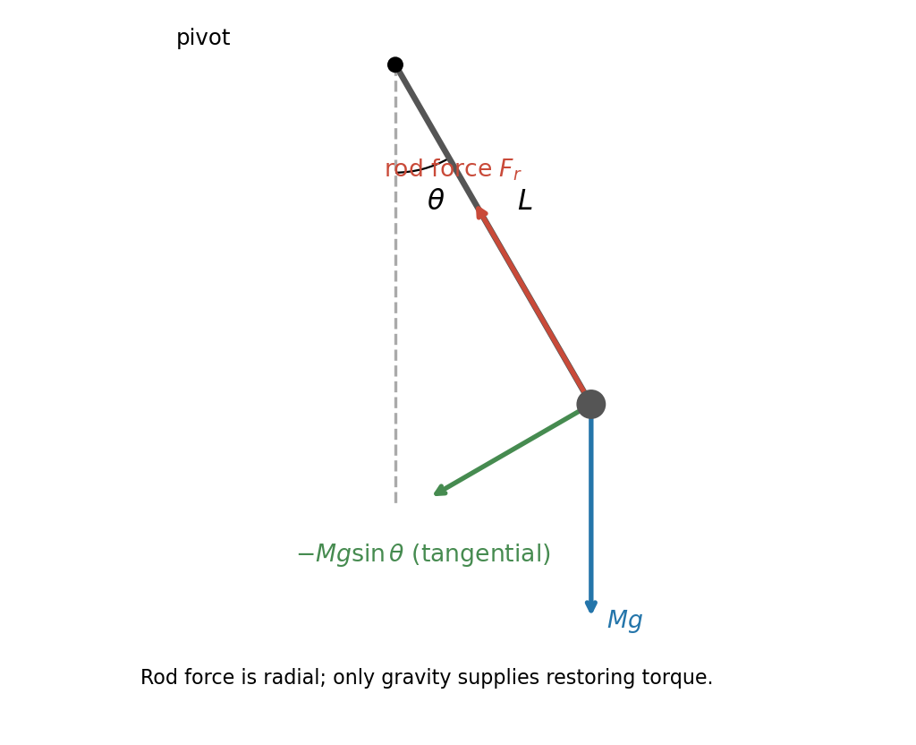
The bob experiences weight vertically downward and a rod force towards the pivot. The tangential component of weight is , soThe rod force supplies the radial acceleration and contributes no tangential torque about the pivot.

To the same small-angle order, writing ,Thus is constant. Put , a signed angular velocity. ThenIf the printed angular speed is intended as the signed rate, set . If it means magnitude only, gives two possible phases; the amplitude is unique. At zero amplitude the phase is arbitrary.
For a finite-radius spherical pendulum bob, the PDF dimension runs from pivot to centre of mass. The parallel axis theorem gives . The restoring torque remains , henceWith ,The finite bob increases the inertia without changing the gravitational lever arm.
In sinusoidal steady state, complex impedance is the voltage phasor divided by the current phasor. Its modulus is the amplitude ratio and its argument is the voltage lead. With the convention, , so .
The PDF labels across , not across the complete driven network. If is the current through , then and , whereThe resistor-referenced parallel-resonator response isWriting ,The maximum occurs at , where and the phase is zero. Below resonance the phase is positive, tending to ; above it the phase is negative, tending to . The amplitude tends to zero at both extremes: the inductor shorts the parallel network at low frequency, and the capacitor does so at high frequency. At resonance their reactive currents cancel, leaving only the resistor current.
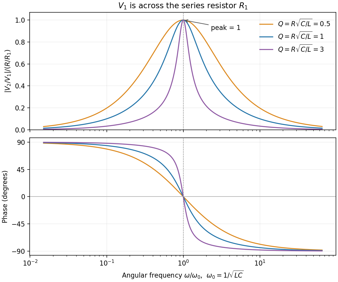
Resistor-referenced parallel-resonator amplitude and phase, normalized without choosing circuit component values
. Details. 
If instead denotes the voltage across the complete circuit, its different transfer ratio is , with peak . This distinction follows directly from the printed voltage endpoints.
For free parallel RLC voltage decay, measure and branch currents from A to B. ThenThere is no external current, so Kirchhoff's current law gives . Differentiating yieldsFor the characteristic equation is . Its underdamped roots giveThe supplied inequality makes real. A real physical voltage has the general form , the real part of the printed complex expression. A general complex-valued solution uses both roots, . The inductor's initial current is fixed consistently by the undifferentiated current balance; it is not an arbitrary additional voltage-mode constant.
Fixed endpoints require , with . Writing ,For equal amplitudes , the two requested profiles areThe first is asymmetric, with an interior zero at ; the second has its interior node at . For two-mode string recurrence, orthogonality means the whole initial profile recurs only when both cosine coefficients equal one. Since ,
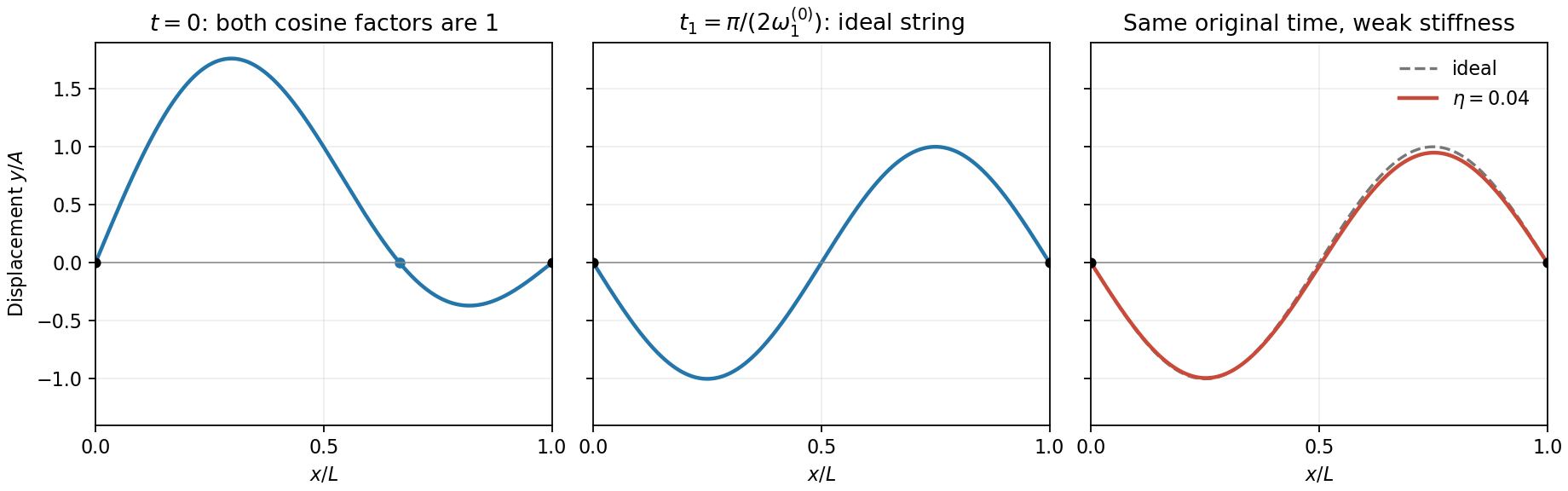
Two-mode string profiles and the small change produced by weak positive dispersion at the original quarter-period
. Details. 
The weak-stiffness string frequency shift follows by expanding the supplied dispersion relation:Higher normal modes acquire larger fractional frequency shifts. Let and retain for the original ideal frequency. At the originally defined time ,Thus the sketch is unchanged, whereas the original quarter-period sketch gains a small negative fundamental component. If is redefined using the new fundamental frequency, its fundamental component is exactly zero and the second-mode change there is only second order. Both conventions agree that generic later shapes change because of relative phase drift.
The new frequency ratio isAn exact recurrence now requires and for integers . If in lowest terms, the first recurrence is ; for irrational there is no exact finite recurrence. Near-recurrences remain possible. Positive stiffness alone does not prove that the ratio is irrational.
Here is potential energy, is the stationary-state total energy eigenvalue, and is its spatial wavefunction. Wavefunction normalization gives , and is the probability of finding the particle in .
A bound state requires . Inside the well the equation is , whereas outside it is , withThe ground state is even and has no node, selecting inside. Normalizability selects decaying, not growing, exterior exponentials. Continuity of and givesThe first excited state, if present, is odd: a sine inside and opposite-sign decaying tails outside. Matching gives . On its first odd branch, , hence . Since , existence requiresThis is the first odd bound-state threshold of a square well. There is no excited bound state below that threshold; equality gives a non-normalizable zero-energy limiting state, not an extra bound state.
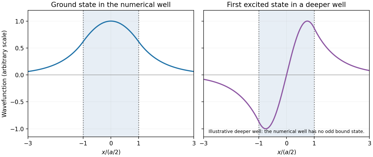
Original finite-well wavefunctions: an even nodeless ground state and an odd excited state in a deeper illustrative well
. Details. 
For the numerical well,The exterior probability of a symmetric finite-well state includes both tails:The threshold is , exceeding the well depth, so there is no excited bound state. The rounded supplied coefficients integrate to rather than exactly one; this rounding does not change the quoted probability precision materially.
For steady currents in vacuum, Ampère's law is . A rectangular loop with one long side inside an ideal long solenoid and the other outside gives , because the exterior field is negligible and the perpendicular sides contribute zero. Thus , approximately uniform away from the ends.
Write the electron electric charge as , with . The Lorentz force is ; it does no work. For perpendicular motion, givesHere is the positive angular speed; the rotation sense is determined by the negative electron electric charge.
The parallel velocity is unaffected, while the perpendicular component rotates. Hence the path is a helix with and . For on-axis entry into a solenoidal tube, the transverse circle passes through that axis: its guiding centre is displaced by , and its maximum distance from the tube axis is , not .
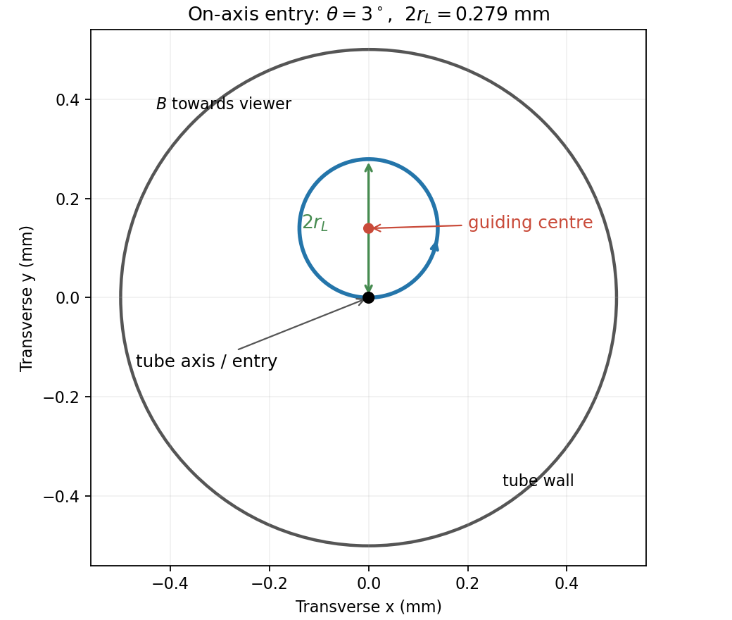
End-on electron orbit: the circle passes through the tube axis and reaches twice its Larmor radius from it
. Details. 
Using the nonrelativistic approximation appropriate to ,The cyclotron period is , so the flight lasts revolutions. The electron therefore crosses the axis again four times before leaving. At , . Wall clearance requires , givingThe transit is longer than a full orbit, so the maximum transverse excursion really is sampled before exit.
For the solenoidal time-of-flight energy window, the prescribed time fixes , while . ThereforeThese are total kinetic energies. The upper value is the ideal grazing limit; if touching the wall counts as rejection, it is a supremum approached from below.
An electric dipole consists of opposite charges separated by a small displacement, with electric dipole moment directed from negative to positive. At distances large compared with its size,The net charge term vanishes; the field decays faster than a monopole field. In an imposed slowly varying electric field,for a permanent fixed dipole. A uniform field produces a torque but no net force. For a linear induced dipole , the interaction energy is instead , because building the dipole also costs energy.
A small planar current loop has magnetic dipole moment , with the normal fixed by the right-hand rule. Outside the source,Magnetic field lines form closed loops; a current-loop dipole does not require magnetic monopoles. Dipole moments describe the leading directional field of a neutral localized source, and their torques explain alignment in external fields.
For two isolated point masses, introduce total mass , reduced mass and relative separation . The relative acceleration is . Conserved specific angular momentum fixes a plane and a constant areal velocity . The specific orbital energy isFor , the trajectory is a conic:Negative energy gives an ellipse, including the circular limit ; zero energy gives a parabola; positive energy gives a hyperbola. Bound ellipses obey andThus Kepler's laws of planetary motion follow from angular momentum conservation and the inverse-square force. For a circular orbit of radius , , while escape from that radius requires . Energy determines whether the orbit is bound; angular momentum also determines its shape. These ideal results neglect extended-body perturbations, drag and relativistic corrections.
In electrostatic equilibrium a conductor has throughout its bulk and constant electric potential on each connected component. Otherwise free charge would continue moving. Gauss's law then excludes bulk excess charge; it resides on surfaces. Just outside a conductor the tangential field vanishes and the normal jump isfor a vacuum interface with outward normal . Surface charge rearranges in an external field to enforce these boundary conditions. Greater curvature often concentrates charge, but the actual distribution is a global boundary-value problem.
An empty closed cavity inside a conductor has constant potential and zero field, even in an external electrostatic field. If a charge is placed in the cavity, a Gaussian surface in the metal shows that the cavity wall carries total induced charge ; its detailed distribution depends on geometry. An initially neutral isolated conductor then has on its exterior surface. A grounded conductor can exchange charge with Earth, so this isolation condition no longer applies.
A useful example is a charge at height above an infinite grounded plane. In the physical half-space, the method of images replaces the induced charges by an image at height , giving the attractive force . The image is a mathematical construction, not an actual charge behind the conductor. Equipotential surfaces and charge conservation determine conductor fields together.
In vacuum, Maxwell's equations in SI units areThe displacement current term makes the last equation consistent with the charge continuity equation. In a source-free region, take the curl of Faraday's law and use . This givesA plane electromagnetic wave therefore propagates at . The divergence equations make both fields transverse; the curl equations giveThe electric fields and magnetic fields are in phase and perpendicular to one another and to the propagation direction. Their energy densities are equal:For electric-field peak amplitude , the time-averaged intensity is . Mutually coupled changing electric fields and magnetic fields transport energy through vacuum, even where no charges or conduction currents are present.
Articles by others on the same topic
There are currently no matching articles.