Past exam of the short options paper of the physics Prelims of the University of Oxford / 2019 (A14119W1)

Source paper: www.whatdotheyknow.com/request/physics_preliminary_past_papers/response/2680788/attach/3/2018%202021%20Physics%20prelims.zip?cookie_passthrough=1

The cover dates this Prelims booklet to 18 June 2019, despite the archive member being filed under 2018/T. These solutions cover its three options independently of the separate Parts A/B booklet.

A complex derivative computed along the real and imaginary directions gives $f^{\prime }=u_x+i{v}_x=v_y-i{u}_y$. Equality yields the Cauchy-Riemann equationsThe gradients satisfy $\nabla u\cdot \nabla v=u_x{v}_x+u_y{v}_y=0$. Since a gradient is normal to a regular level set, the two families meet at right angles by orthogonality wherever $f^{\prime }\ne 0$. At a critical point the regular-curve argument fails: for $f=z^2$ both gradients vanish at zero, so the assertion requires this qualification.

Set $A=x^2-y^2$ and $B=2xy$. Direct differentiation givesTheir sum vanishes, proving that $u$ is a harmonic function. More generally the Cauchy-Riemann equations give $u_{xx}+u_{yy}=v_{yx}-v_{xy}=0$ and $v_{xx}+v_{yy}=-u_{yx}+u_{xy}=0$; the mixed partial derivatives commute because a holomorphic function is smooth. Since $e^{i{z}^2}=e^{-B}(\cos A+i\sin A)$, a harmonic conjugate and the resulting holomorphic function areThese expressions also verify the Cauchy-Riemann equations directly.

The chain rule in polar coordinates gives $u_r=u_x\cos \theta +u_y\sin \theta$ and $u_{\theta }=r(-u_x\sin \theta +u_y\cos \theta )$, with analogous expressions for $v$. Substituting the Cauchy-Riemann equations givesThe restriction excludes the coordinate singularity at the origin.

Choose a continuous branch of a multivalued function of the complex logarithm on a simply connected region avoiding zero. ThenAlternatively $u_r=-e^{-\theta }\sin (\ln r)/r=v_{\theta }/r$ and $v_r=e^{-\theta }\cos (\ln r)/r=-u_{\theta }/r$, verifying the Cauchy-Riemann equations. The holomorphy is local to a chosen branch of a multivalued function: increasing $\theta$ by $2\pi$ multiplies $g$ by $e^{-2\pi }$, so this is not a single-valued holomorphic function on the whole punctured plane.

For $n\ge 1$, $f=z^n{e}^{n/z}$ is holomorphic at every finite nonzero point. At zero its Laurent series has infinitely many negative powers, so zero is an essential singularity. If the Riemann sphere is included, $f(1/w)=w^{-n}{e}^{nw}$ has a pole of order $n$ at $w=0$, so infinity is a pole of order $n$.

Expanding the exponential function produces the Laurent seriesIn particular its residue is $a_{-1}=n^{n+1}/(n+1)!$.

For a positively oriented circle of any radius $R>0$, the residue theorem givesOnly the $z^{-1}$ coefficient in the Laurent series contributes. Reversing the orientation changes the sign.

If $f(z)=\sum a_j{z}^j$, then $f(-z)=\sum (-1{)}^j{a}_j{z}^j$ and its residue at zero is $-a_{-1}$. The circle $|z-1|=2$ encloses zero and no other finite singularity. Thus the residue theorem givesfor positive orientation.

Cauchy's integral theorem states that a holomorphic function on a simply connected open region has zero contour integral around every closed piecewise smooth contour in that region. More generally the same holds for a contour homologous to zero in its domain of holomorphy. Having no singularity on the curve alone is insufficient: $1/z$ has a nonzero contour integral around the unit circle.

Put $z=e^{i\theta }$, so $d\theta =dz/(iz)$, $\cos 2\theta =(z^2+z^{-2})/2$ and ${\cos }^{2}3\theta =(z^6+2+z^{-6})/4$. The contour integral isThe enclosed poles are $0$ and $\pm 1/\sqrt{2}$. For the rational function displayed without the prefactor $1/(4i)$, the residue at zero is $-21/8$ and the two other residues sum to $27/8$. Therefore the residue theorem givesA useful independent check is the Fourier series $(5-4\cos \varphi {)}^{-1}=\frac{1}{3}[1+2{\sum }_{k\ge 1}{2}^{-k}\cos k\varphi ]$; only its constant and third Fourier coefficients survive.

The square root produces branch points at $z=\pm 1$, with local behaviour proportional to $(z\mp 1{)}^{-1/2}$. One branch cut can join them along $[-1,1]$. Another choice uses the two rays $(-\infty ,-1]\cup [1,\infty )$. Each choice prevents a loop from enclosing just one branch point within a single-valued domain. For the finite-segment choice fix $\sqrt{z^2-1}\sim z$ at infinity. Infinity is then a pole of order three, not a branch point, since

Use the branch cut $[-1,1]$ and the branch of a multivalued function normalized by $\sqrt{z^2-1}\sim z$. The Laurent series from the preceding solution has $z^{-1}$ coefficient $3/8$. Consequently every sufficiently large positively oriented circle givesAlthough $f$ grows cubically, its other Laurent series terms have zero contour integral. Choosing the opposite branch of a multivalued function reverses the sign; neither the branch of a multivalued function nor the orientation can be omitted from the answer.

Shrink the positive outer contour to the branch cut $[-1,1]$. On its upper bank the chosen branch of a multivalued function has $\sqrt{x^2-1}=i\sqrt{1-x^2}$ and on the lower bank it has the negative of this value. The upper bank runs from $1$ to $-1$, and the lower bank runs from $-1$ to $1$. The endpoint circles contribute $O(\sqrt{ϵ})$ and vanish. HenceThe change of variables $x=\sin t$ independently reduces the result to the integral of ${\sin }^{4}t$ over $[-\pi /2,\pi /2]$.

Kepler's third law for two point masses in a Newtonian gravitational field isHere $a$ is the semimajor axis of their relative orbit, $P$ the orbital period and $G$ the gravitational constant. Equivalently $(P/\mathrm{yr}{)}^2=(a/\mathrm{AU}{)}^3/[(M_1+M_2)/M_{\odot }]$, to the accuracy with which these astronomical units normalize the solar mass.

Assume a circular orbit and an orbital inclination $i\simeq 90^{\circ }$, as appropriate for a simple eclipsing binary estimate. At quadrature the two radial velocities are opposite and equal to the orbital speeds. The more massive component has the smaller amplitude. With the centre of mass as origin,Thus $a_1=0.1103\mathrm{AU}$, $a_2=0.2206\mathrm{AU}$ and Kepler's third law givesThe orbital plane contains the observer's line of sight; at quadrature the two velocities point towards and away from that observer, as labelled in the original schematic below. For an elliptic orbit, the measured amplitudes instead give $a\sin i=P(K_1+K_2)\sqrt{1-e^2}/(2\pi )$; the numerical answer requires the circular assumption.

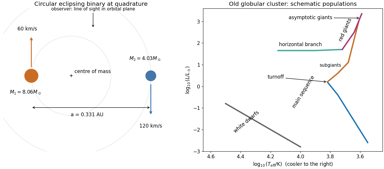
Adopt the approximate mass-luminosity relation $L/L_{\odot }\simeq (M/M_{\odot }{)}^3$ and equal available fuel fractions. The main-sequence lifetime then scales as $M/L$, givingUsing an exponent $3.5$ instead gives about $5.4\times 10^7$ and $3.1\times 10^8$ years; these are model-dependent estimates. At $r=3r_s=6GM/c^2$ the Newtonian gravitational potential energy released from infinity is $GMm/r=m{c}^2/6$. Half remains as kinetic energy in a circular orbit, so the radiatable binding energy is $GMm/(2r)$:Using the whole potential energy loss would give $1/6$, which does not subtract the final kinetic energy. A fully relativistic calculation for a nonrotating black hole gives $1-\sqrt{8/9}\simeq 5.7\%$. When the surviving star exhausts hydrogen burning, it expands off the main sequence and can fill its Roche lobe. Binary mass transfer to the black hole can form an accretion disk and an X-ray binary; unstable binary mass transfer may instead produce a common envelope. This is conditional on the binary star remaining bound after the first remnant forms. The supplied black hole endpoint is an assumption, not a universal outcome for an isolated $8M_{\odot }$ star.

A thin spherical shell has outward pressure force $-4\pi r^2(dP/dr)dr$ and inward gravitational force $GM(r)4\pi r^2\rho (r)dr/r^2$. Hydrostatic equilibrium requiresA uniform-density solar model gives $M(r)=M_{\odot }(r/R_{\odot }{)}^3$, $\bar{\rho }=3M_{\odot }/(4\pi R_{\odot }^3)$, and after integration from $R_{\odot }$ to zero,Thus the appropriate orders of magnitude are $10^{14}$–$10^{16}\mathrm{Pa}$ and $10^7\mathrm{K}$. The uniform-density approximation underestimates the actual central pressure because the Sun is centrally concentrated. Radiation pressure is neglected in applying the ideal gas law.

A free-fall timescale estimate follows from $R/t^2\sim GM/R^2$:Falling to a central point mass gives the more precise factor $\pi /(2\sqrt{2})$, or $1.77\times 10^3\mathrm{s}$; a distributed star changes an order-one coefficient. For any spherical mass distribution with radius $R$,The inequality is strict for an extended star; equality is approached by a thin shell at $R$. For an monatomic gas the virial theorem is $2U+\Omega =0$, so half the gravitational potential energy released by contraction heats the star and half can be radiated. The Kelvin-Helmholtz cooling time is therefore of orderA uniform-density model gives $3G{M}^2/(10RL)\simeq 9.4\times 10^6\mathrm{yr}$. The given bound fixes a scale, rather than an exact contraction history; both estimates are far shorter than the Sun's main-sequence lifetime.

The right panel of the figure in solution has luminosity increasing upwards and effective temperature decreasing to the right. An old globular cluster contains a low-mass main sequence, a main-sequence turnoff, subgiants, a red giant branch, a horizontal branch, an Asymptotic giant branch and a faint hot white dwarf sequence. Its high-mass main sequence is absent because those stars have evolved.

If a fraction $f_c=0.1$ of the star participates in hydrogen burning, with initial hydrogen mass fraction $X=0.7$, the available nuclear binding energy is $0.007f_{c}XM{c}^2$. Assuming a roughly constant luminosity and coeval stars,Taking the quoted core fraction as hydrogen fuel itself, $f_{c}X=0.1$, gives $1.98\times 10^{10}\mathrm{yr}$. Stating the fuel convention matters: burning the whole stellar mass overestimates the age by about an order of magnitude. Evolving luminosity and detailed stellar structure are needed for an accurate age.

The Milky Way has a thin stellar galactic disk, radius roughly $15$–$20\mathrm{kpc}$ and scale height about $0.3\mathrm{kpc}$, containing gas, dust, young and old stars, spiral arms and most current star formation. Its stellar mass is a few $10^{10}{M}_{\odot }$. A thicker, older galactic disk has scale height around $1\mathrm{kpc}$ and stellar mass of order $10^{10}{M}_{\odot }$, with little cold gas.

The central galactic bulge and bar extend a few thousand parsecs and contain about $10^{10}{M}_{\odot }$, largely older stars. The central supermassive black hole has mass about $4\times 10^6{M}_{\odot }$ and is negligible in the total galactic budget. A diffuse old metal-poor stellar halo, extending tens to over $100\mathrm{kpc}$, contains globular clusters and roughly $10^9{M}_{\odot }$ in stars. An extended dark matter halo reaches roughly $200\mathrm{kpc}$ and dominates the total mass, of order $10^{12}{M}_{\odot }$. These are approximate component scales; the gaseous galactic halo also extends beyond the stellar galactic disk.

Treat the gravitational field as approximately spherical. The circular orbit condition givesIf every star had a representative mass $m$ and obeyed $L/L_{\odot }=(m/M_{\odot }{)}^3$, its mass-to-light ratio would be $(m/M_{\odot }{)}^{-2}$, giving $\boxed{m\simeq 0.47M_{\odot }}$. This is a one-mass estimate, not an actual average inferred uniquely from the data: a galactic stellar mass function, stellar remnants, dust and nonstellar mass alter the relation. The flattening of the galactic disk also changes the spherical conversion by an order-one factor.

Assume an isotropic, stationary spherical galaxy cluster. Its three-dimensional velocity dispersion obeys $⟨v^2⟩=3{\sigma }_{\mathrm{los}}^2$. For a uniform sphere, the virial theorem gives $3M{\sigma }_{\mathrm{los}}^2=3G{M}^2/(5R)$, henceA different density profile changes the coefficient, so $10^{15}{M}_{\odot }$ is the meaningful scale. For isothermal X-ray gas in hydrostatic equilibrium,Using $\mu =0.6$ and a representative slope $-d\ln {\rho }_g/d\ln r=2$–$3$ at $1\mathrm{Mpc}$ gives $M_X\simeq (1.3$–$1.9)\times 10^{15}{M}_{\odot }$. The temperature and extent alone cannot fix this coefficient without a density profile. The total luminosity is $5\times 10^{12}{L}_{\odot }$, so the previously inferred mass-to-light ratio gives

Three physically distinct contributions are unseen dark matter, hot diffuse intracluster gas omitted from the summed stellar mass, and faint stars or stellar remnants missed by transferring the Milky Way mass-to-light ratio to the cluster. The first two are actual additional components; the third changes the inferred stellar budget. Departures from virial equilibrium, velocity anisotropy or extra nonthermal pressure can also bias the dynamical or X-ray estimates, although they need not remove the discrepancy.

A blackbody is an ideal body that absorbs all incident electromagnetic radiation, at every frequency and direction. Its absorptivity is one, so Kirchhoff's law of thermal radiation makes its equilibrium emissivity one as well. At a specified temperature its thermal spectrum is universal: it depends on temperature, not material or shape. This does not mean it looks black when hot; it can glow brightly while remaining a perfect absorber.

A small hole in a nearly isothermal opaque cavity approximates a blackbody, because radiation entering the hole undergoes many interactions before it could escape. In thermal equilibrium the cavity contains an approximately isotropic Planck spectrum. The emitted radiance follows Planck's law, its integrated outward radiant exitance follows the Stefan–Boltzmann law, and its wavelength peak follows Wien's displacement law. A real surface can have wavelength- and direction-dependent emissivity below this ideal limit.

The constants are the Planck constant $h$, photon frequency $\nu$, speed of light $c$, Boltzmann constant $k_B$ and absolute temperature $T$. The supplied $U_{\nu }$ is a spectral energy density, with units $\mathrm{J}{\mathrm{m}}^{-3}\mathrm{H}{\mathrm{z}}^{-1}$. It describes equilibrium radiation per volume and frequency interval, rather than emitted power itself. For isotropic cavity radiation the corresponding surface spectral radiant exitance is $M_{\nu }=c{U}_{\nu }/4$.

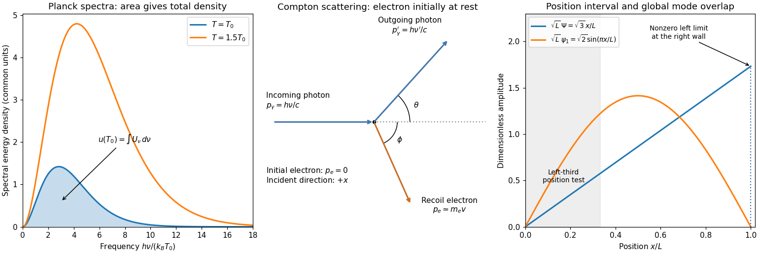
At low frequency the curve rises as ${\nu }^2$; it has one positive maximum and an exponentially decaying high-frequency tail. The left panel below shades the area $u(T)={\int }_0^{\infty }{U}_{\nu }d\nu$ under one curve. Put $x=h\nu /(k_{B}T)$; thenThe remaining dimensionless integral is independent of temperature, soThus doubling temperature doubles the characteristic frequency scale, raises the spectrum's height by eight and increases its area by sixteen. Total emitted energy also depends on emitting area and elapsed time.

For $x=h\nu /(k_{B}T)\ll 1$, the Taylor expansion $e^x-1=x+O(x^2)$ gives the Rayleigh-Jeans law for equilibrium radiation,This is the classical limit: each electromagnetic mode has mean thermal energy approximately $k_{B}T$. Extending it to arbitrarily large frequencies would give a divergent integrated energy density, the ultraviolet catastrophe.

For $x\gg 1$, $e^x-1\simeq e^x$, giving the Wien approximationPlanck's quantum hypothesis assigns equally spaced mode energies $E_n=nh\nu$. When the spacing is small relative to $k_{B}T$, many levels are occupied and the classical approximation works. When $h\nu \gg k_{B}T$, exciting even one quantum is exponentially unlikely, suppressing the high-frequency tail. The single expression $⟨E⟩=h\nu /(e^x-1)$ contains both limits. Comparing temperature directly to $h\nu$ would be dimensionally incorrect; the low-temperature condition means $k_{B}T\ll h\nu$.

First convert from a spectral energy density per unit frequency to one per unit wavelength, including the Jacobian matrix and determinant:Set $d{U}_{\lambda }/d\lambda =0$ and define $x=hc/(\lambda k_{B}T)$. The nonzero maximum satisfies $5(1-e^{-x})=x$, with numerical root $x=4.96511$. ConsequentlyThis is Wien's displacement law. One must maximize the wavelength density, rather than find the frequency maximum and merely put $\lambda =c/{\nu }_{\max }$: the frequency and wavelength peaks of Planck's law are different because a spectral density changes under a change of coordinate.

Using the stipulated $570\mathrm{nm}$ as a wavelength-density peak, Wien's displacement law givesThis is a rough estimate from the supplied characteristic wavelength, not an accurate measurement of the Sun's effective temperature. The Sun emits a broad, approximately thermal visible spectrum and appears white outside the atmosphere; its familiar yellow appearance does not identify a monochromatic thermal peak. A photospheric effective temperature near $5770\mathrm{K}$ instead corresponds to a wavelength-density maximum near $502\mathrm{nm}$.^[ref][ref]

The core must be much hotter to provide the pressure required for hydrostatic equilibrium and to sustain nuclear fusion. Outward energy transport through an opaque interior proceeds down a temperature gradient, by radiative diffusion and then convection through much of the outer envelope. The observable photosphere radiates to space at the temperature needed to carry the solar luminosity, $L_{\odot }=4\pi R_{\odot }^2\sigma T_{\mathrm{eff}}^4$; it is not an unobstructed view of the hot core. The printed core estimate above $20$ million degrees is also too high for the present Sun: the standard central temperature is about $1.56\times 10^7\mathrm{K}$. This correction leaves the large core-to-surface contrast and its explanation intact.^[ref]

Compton scattering transfers energy and momentum from a photon to an electron. For an initially stationary, approximately free electron, a photon scattered through a nonzero angle generally has lower frequency and longer wavelength; the recoiling electron carries the difference. The effect demonstrates the photon momentum $p_{\gamma }=h\nu /c=h/\lambda$, beyond a purely elastic classical scattering description.

The middle panel of the figure in solution shows the incident photon along $+x$, the outgoing photon at angle $\theta$ above that direction, and the recoiling electron at deflection angle $\varphi$ below it. Each arrow labels its particle and momentum; the initial electron is at rest at the interaction point. The scattered photon and electron have opposite transverse momentum components, while their forward components sum to the incident photon momentum.

Take a stationary initial electron of mass $m_e$, a photon incident along $x$, and a nonrelativistic recoil velocity of magnitude $v$. Choose $\theta$ above $x$ for the scattered photon and $\varphi$ below $x$ for the electron. Conservation of momentum givesThe electron's unchanged rest energy cancels in conservation of energy, leavingEquivalently use $h\nu /c=h/\lambda$ and $h\nu =hc/\lambda$. The nonrelativistic limit requires $v/c\ll 1$, and treating the electron as free requires its binding energy to be negligible on the scale of the collision.

For complete photon backscatter $\theta =\pi$, the electron recoils forward and momentum conservation givesCombining this with conservation of energy and writing $\Delta \lambda ={\lambda }^{\prime }-\lambda$ givesFor $\Delta \lambda \ll \lambda ,{\lambda }^{\prime }$, the final ratio is approximately four, soWithin the stated nonrelativistic equations the unsimplified relation is implicit and has higher-order recoil corrections; the displayed final approximation is all that the small-shift assumption supports. Exact relativistic Compton recoil kinematics gives $\Delta \lambda =(h/m_{e}c)(1-\cos \theta )$, and therefore exactly $2{\lambda }_C$ at backscatter. Agreement at leading order does not make the nonrelativistic derivation exact at arbitrary photon energy.

The ordinary electron Compton wavelength isA photon of that wavelength has energy equal to the electron rest energy, $hc/{\lambda }_C=m_e{c}^2$. It therefore sets the characteristic scale at which photon recoil cannot generally be treated nonrelativistically, and it sets the magnitude of the Compton wavelength shift. The reduced Compton wavelength, ${\bar{\lambda }}_C=\hslash /(m_{e}c)={\lambda }_C/(2\pi )$, is a related but different convention. Localization on this reduced scale needs momenta of order $m_{e}c$, so a nonrelativistic single-particle description becomes inadequate. Neither wavelength is a measured geometrical radius of the electron.

Retain the backscattering geometry from part (c). With $\lambda =10\mathrm{nm}$, ${\lambda }^{\prime }=\lambda +2{\lambda }_C$ differs from $\lambda$ by only $4.85\times 10^{-4}$ of its value. Momentum conservation givesThe Lorentz-factor correction is of order $v^2/c^2\simeq 2.4\times 10^{-7}$, so the electron recoil is safely nonrelativistic. Its kinetic energy is only about $0.060\mathrm{eV}$, compared with incoming photon energy about $124\mathrm{eV}$. This validates the free-electron recoil approximation's relativistic aspect; actual binding or thermal motion in matter can require separate corrections. No larger recoil occurs at another scattering angle for the same initial photon.

Inside the infinite square well, $V=0$, and the time-independent Schrödinger equation isFor $E>0$, write $k^2=2mE/{\hslash }^2$ and $\psi =A\sin kx+B\cos kx$. The first Dirichlet boundary condition gives $B=0$, and the second requires $kL=n\pi$ for a nonzero state. The case $n=0$ is identically zero; negative $n$ only changes an overall quantum phase. For $E=0$ a linear solution satisfying both walls is zero, and for $E<0$ the hyperbolic solutions likewise cannot satisfy both walls nontrivially.

Wavefunction normalization, ${\int }_0^L|\psi {|}^{2}dx=1$, fixes $|A|=\sqrt{2/L}$. The orthonormal energy eigenstates and energy eigenvalues are thereforeEach state vanishes outside the well. Its stationary time-dependent form is ${\Psi }_n(x,t)={\psi }_n(x)e^{-i{E}_{n}t/\hslash }$. General states are normalized superpositions of these modes, rather than additional single energy eigenstates.

Assume the given wavefunction is zero outside $[0,L]$. Wavefunction normalization requiresAn arbitrary overall quantum phase is unobservable, so choose the positive real representative $N=\sqrt{3}/L^{3/2}$.

The linear ramp state in an infinite square well has a boundary subtlety: the limiting value at $L$ is $\sqrt{3/L}$, rather than zero. The function is still a normalized element of the well's Hilbert space $L^2(0,L)$, so position measurement and energy-projection probabilities are meaningful. It is not in the domain of the Dirichlet Hamiltonian, nor is it a finite-energy box state. Altering the value at the single endpoint does not cure its nonzero boundary trace; a physical finite-energy preparation must smooth the function to zero near the wall. The following probabilities refer to the supplied idealized state.

Apply the position version of the Born rule to the normalized wavefunction:The result is independent of $L$ because the state and the measurement interval scale together. Most position probability lies towards the right wall, since the probability density grows as $x^2$.

An energy measurement selects the ground state with probability equal to the squared inner product with ${\psi }_1$. Using $N=\sqrt{3}/L^{3/2}$ and integration by parts,ThusThe full Fourier sine series has $c_n=(-1{)}^{n+1}\sqrt{6}/(n\pi )$, so ${\sum }_n|c_n{|}^2=(6/{\pi }^2){\sum }_n{n}^{-2}=1$, an independent wavefunction normalization check. However $E_n|c_n{|}^2=3{\hslash }^2/(m{L}^2)$ for every $n$, hence ${\sum }_n{E}_n|c_n{|}^2$ diverges. This explicitly verifies the infinite-energy expectation qualification in part (b), without invalidating the individual projection probabilities.

The two probabilities concern different quantum measurements, so there is no requirement that they match or that one bound the other. The spatial interval $[0,L/3]$ contains little of the state: its probability density is smallest near zero and increases towards $L$. By contrast, the positive ground state extends across the whole well. It has substantial same-sign overlap with the positive linear wavefunction, with no cancellation between lobes in the overlap integral. The right panel of the figure in solution illustrates these two amplitudes and marks the small position interval.

Consequently a large global ground-state probability can coexist with a small probability of finding the particle in the left third. This is not because the ground state is spatially confined to that third; a ground-state particle can be found throughout the well. In operator language the two events are projections onto a spatial subspace and onto one energy eigenstate, respectively.