Past exam of the short options paper of the physics Prelims of the University of Oxford

Source: www.whatdotheyknow.com/request/physics_preliminary_past_papers/response/2680788/attach/3/2018%202021%20Physics%20prelims.zip?cookie_passthrough=1

Singularities. The complex exponential factors as $F(z)=e^{z/2}{e}^{1/(2z)}$. The second factor has an essential singularity at zero, and multiplication by the nonvanishing holomorphic function $e^{z/2}$ does not remove it. There are no other finite singularities. On the Riemann sphere, infinity is also an essential singularity, since $F(1/\zeta )=F(\zeta )$.

Symmetry and integral formula. The identity $F(1/z)=F(z)$ and uniqueness of the Laurent series on $0<|z|<\infty$ give $F_{-k}=F_k$ for every integer $k$. The Laurent coefficient formula, on the positively oriented unit circle, givesThe imaginary part vanishes by the substitution $\theta \mapsto 2\pi -\theta$. Hence

Polynomial contour integral. For an integer $n\ge 0$ and integer $p$, the binomial theorem gives $(1+z^2{)}^n={\sum }_{j=0}^n(\genfrac{}{}{0ex}{}{n}{j})z^{2j}$. The residue theorem selects $2j-n-p-1=-1$, that is $j=(n+p)/2$. Therefore the correct complete statement isThe printed nonnegative-integer condition alone misses $j\le n$. For example $n=0,p=2$ satisfies that condition, but the integral is zero and the displayed factorial $(-1)!$ is undefined.

Explicit coefficients. Both Taylor series inconverge absolutely and uniformly on every compact annulus away from zero, so their product can be regrouped. For $k\ge 0$, put $r=s+k$ and $s=m$. For arbitrary integer $k$, use the already proved symmetry:Here $I_j$ is a modified Bessel function. The printed series is directly meaningful for $k\ge 0$; for negative $k$ the absolute values, or an appropriately shifted lower summation limit, are essential.

Conformality and analyticity. Use the orientation-preserving convention for a conformal map, with a continuously differentiable, nonzero differential. Its Jacobian matrix must be a positive scale times a rotation,Thus $u_x=v_y$, $u_y=-v_x$, the Cauchy-Riemann equations; continuous partial derivatives then imply that $u+iv$ is a holomorphic function. If angle preservation is allowed to reverse orientation, the statement needs this qualification: $z\mapsto \bar{z}$ preserves unsigned angles but is an anticonformal map and is not a holomorphic function.

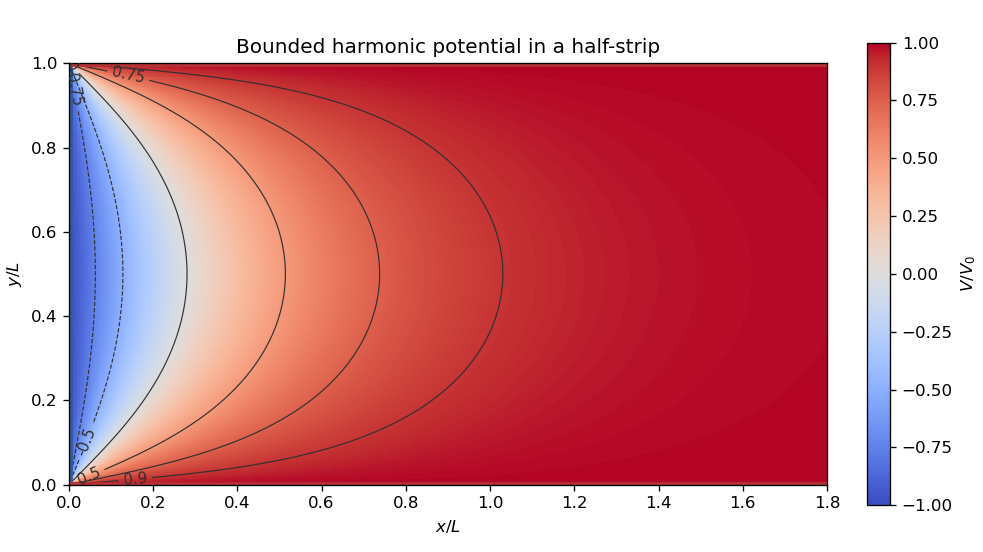
The mapping. Put $a=\pi /L$. The displayed components combine to giveIts derivative does not vanish in the open half-strip $x>0$, $0<y<L$, so it is a conformal map there. Also $\mathrm{Im}w=\sinh (ax)\sin (ay)>0$. The lower edge maps to $[1,\infty )$, the upper edge to $(-\infty ,-1]$, and the vertical edge to $[-1,1]$. The open half-strip maps bijectively onto the upper half-plane. Indeed, $\cosh \zeta =\cosh \eta$ implies $\zeta =\pm \eta +2\pi im$; the half-strip allows only equality. Surjectivity follows by solving $t+t^{-1}=2w$ and choosing the root $t=e^{az}$ with $|t|>1$ and $0<\arg t<\pi$. The two corners are boundary critical points, not interior failures of conformality.

Transformed boundary values. A conformal map preserves Laplace's equation up to a positive scale. Thus the transformed Dirichlet problem is to find a real harmonic function $U(u,v)$ on $v>0$ withThe conflicting values at the original corners are interpreted as one-sided edge limits.

Logarithmic solution. Choose the complex logarithms of $w\pm 1$ with arguments between zero and $\pi$ in the upper half-plane. A linear combination $F(w)=\alpha \log (w+1)+\beta \log (w-1)+\gamma$ is a complex-valued harmonic function, since it is a holomorphic function; the real physical potential must be a real or imaginary part. In particular, setThenOn the three real boundary intervals, the argument difference is respectively $0,\pi ,0$, which gives the required values. This is the bounded harmonic solution, with $U\to V_0$ at infinity; uniqueness holds in this bounded class by the maximum principle. Without a boundedness or far-field condition, the edge data alone do not give uniqueness: one may add $C\sinh (\pi x/L)\sin (\pi y/L)$.

Back substitution. Sincethe required continuous argument difference is $2\arctan [\sin (ay)/\sinh (ax)]$ in the open half-strip. ConsequentlyAs $y\to 0,L$ with $x>0$, the arctangent tends to zero; as $x\to 0^{+}$ with $0<y<L$, it tends to $\pi /2$. These limits verify every open edge of the Dirichlet problem.

Singularities and cuts. There are four simple poles $z_j=e^{i(\pi /4+j\pi /2)}$, $j=0,1,2,3$, because the roots of $1+z^4$ are simple and do not coincide with $\pm 1$. At $z=\pm 1$, the local behavior is a nonzero constant times $(z\mp 1{)}^{-1/2}$: these are square-root branch points. Infinity is not a branch point; on either branch $f(z)=O(z^{-5})$, so it extends there with a zero of order five. Three valid choices of branch cuts are the segment $[-1,1]$, the two rays $(-\infty ,-1]\cup [1,\infty )$ joined through infinity, or a semicircular arc joining $-1$ to $1$ and avoiding the poles. A circuit about either endpoint changes the sign, while a circuit about both endpoints does not.

Branch and residues. On $\mathbb{C}\setminus [-1,1]$, let $s(z)=\sqrt{z^2-1}$ be the branch with $s(z)/z\to 1$ at infinity, and define $\sqrt{1-z^2}=-is(z)$. Its upper boundary value on $(-1,1)$ is positive. The residue at a simple pole $z_j$ isFor fully explicit values, putIn counterclockwise order $z_0,z_1,z_2,z_3$, the values of $s$ are $A+iB,-A+iB,-A-iB,A-iB$. Since $A^2+B^2=\sqrt{2}$, substitution yieldsA branch point has no ordinary residue, since it has no single-valued Laurent series on a punctured neighborhood. At infinity the residue is zero.

Contour evaluation. The original contour goes counterclockwise around a large circle and clockwise round the slit, with its upper lip directed to the right. The large-circle contribution is $O(R^{-4})$. Small endpoint arcs contribute $O({ϵ}^{1/2})$. The artificial slit extension from $1$ to $R$ has equal boundary values on both sides, so its contributions cancel. On $(-1,1)$ the two boundary values of $f$ are opposite. Thus, with $I$ denoting the requested real integral, the residue theorem givesTherefore

Assume spherical stars, central eclipses, uniform disc surface brightness, and negligible third light. Let $s$ denote the smaller star and $\ell$ the larger one, with $r=R_s/R_{\ell }\le 1$ and ${\ell }_s=L_s/L_{\ell }$. Normalize the out-of-eclipse flux to one, and denote the deep and shallow fractional losses by $D$ and $d$. The graph gives approximately $F_{\mathrm{out}}\simeq 0.98$, $F_{\mathrm{deep}}\simeq 0.57$, $F_{\mathrm{shallow}}\simeq 0.90$, so $D\simeq 0.42$, $d\simeq 0.08$; the last digits are graphical estimates.

At total occultation of the smaller star, the lost flux is $L_s/(L_s+L_{\ell })$. At its central transit across the larger star, the lost flux is $r^2{L}_{\ell }/(L_s+L_{\ell })$. There are two identifications:

These are ratios of luminosities in the observed band. Treating them as bolometric luminosities requires similar band corrections or an explicitly bolometric light curve. Limb darkening and finite exposure times limit the precision of these elementary estimates.

The Stefan–Boltzmann law gives $L=4\pi R^2\sigma T_{\mathrm{eff}}^4$ for bolometric luminosity. HenceWith the central values above, this is approximately $1.51$ for the first geometry and $0.67$ for the second. If only one-band luminosities are measured, bolometric corrections are needed before using this formula for effective temperatures.

Two direct methods are fitting the continuum stellar spectrum or several photometric colors to a stellar atmosphere model, and measuring temperature-sensitive absorption lines or line ratios in a stellar spectrum. The former includes the approximate black-body radiation estimate ${\lambda }_{\max }T=b$ from Wien's displacement law; the latter uses ionization and excitation populations. Observations during total eclipse or spectral disentangling help separate the two stellar spectra.

For comparable composition and accessible fuel fractions, the main-sequence lifetime is proportional to available nuclear fuel divided by luminosity, $t_{\mathrm{MS}}\propto M/L$. Estimate the masses from a calibrated mass-luminosity relation $L\propto M^{\alpha }$ in the appropriate mass range. ThenFor illustration $\alpha =3.5$ gives about $1.27$ and $5.6$ for the two graphical luminosity ratios. The common main sequence approximation is additional physics; eclipse depths alone do not determine masses or ages. A main sequence consistency check would also favor the second geometry because ordinary main-sequence stars have radius and effective temperature increasing with mass.

Let $r$ be radial position, $\mathcal{F}=L/(4\pi r^2)$ the outward radiative energy flux, and $P_r=a{T}^4/3$ the radiation pressure. A thin layer absorbs a fraction $\kappa \rho dr$ of an incident directed beam. Since a photon carries momentum $E/c$, the outward force per unit volume deposited by the radiation is $\kappa \rho \mathcal{F}/c$. Balance it against the radiation pressure gradient:Substituting $d{P}_r/dr=(4a/3)T^{3}dT/dr$ yields the radiative diffusion equationThe sign expresses outward energy flux down the temperature gradient. The approximation assumes optically thick material and near local thermodynamic equilibrium, with an appropriate mean opacity.

The printed attenuation law describes the loss from an incident beam; it is not generally the radial derivative of the net luminosity, since absorption is accompanied by emission. For a concrete counterexample, in a steady envelope without local energy generation the net luminosity is constant even though $\kappa \rho >0$ and $dT/dr<0$. Applying $dL/dr=-\kappa \rho L$ to that net luminosity would contradict energy conservation. The local momentum deposition argument supplies the physically correct derivation.

Write $m(r)$ for enclosed mass. The stellar hydrostatic equation is $dP/dr=-Gm\rho /r^2$. If radiation pressure dominates, compare it directly with the radiative diffusion result for $d{P}_r/dr$:This is the limiting Eddington luminosity scaling, assuming fixed composition and electron-scattering opacity.

If gas pressure dominates, use stellar homology: characteristic density $\rho \sim M/R_{\ast }^3$ and pressure $P\sim G{M}^2/R_{\ast }^4$. The ideal gas law then givesEstimating $|dT/dr|\sim T/R_{\ast }$ in radiative diffusion givesThus at fixed $\mu$ and constant electron-scattering opacity, $\boxed{L\propto M^3}$. These are stellar homology estimates for radiative stars, not exact relations valid for arbitrary composition and internal transport.

The same gas-pressure stellar homology estimates give $T\propto \mu M/R_{\ast }$ and $\rho \propto M/R_{\ast }^3$. With Kramers' opacity law $\kappa \propto \rho T^{-7/2}$, radiative diffusion givesConsequently the claimed exponent five additionally requires the approximate low-mass main-sequence mass-radius relation $R_{\ast }\propto M$ and fixed composition:The supplied opacity and pressure assumptions alone do not establish that mass-radius relation. For example, a homologous fixed-radius family obeys those scaling assumptions but gives $L\propto M^{11/2}$, not $M^5$. More generally $R_{\ast }\propto M^q$ gives $L\propto M^{(11-q)/2}$. Very low-mass stars can be convective, where this radiative model ceases to apply.

Use ${\rho }_r,{\rho }_m$ as energy per volume, as specified in the prose, and let $R$ have dimensions of length so that the positive curvature magnitude $k$ is dimensionless. The Friedmann equation for spatial curvature $-k$ isFor an energy density the cosmological perfect-fluid continuity equation is $\dot{\rho }+3H(\rho +P)=0$. Nonrelativistic matter has negligible pressure and radiation has $P_r={\rho }_r/3$. Thus the four contributions to $H^2$ scale respectively asFor nonzero positive densities and $\Lambda >0$, the usual possible sequence is radiation domination, matter domination, curvature domination, then cosmological-constant domination. A distinct era for each is not guaranteed: coefficients may cause curvature to be overtaken by the cosmological constant before it ever dominates. If $\Lambda =0$, curvature dominates asymptotically; negative $\Lambda$ does not give a late positive vacuum-dominated expansion.

The printed auxiliary relation $P_r={\rho }_r{c}^2/3$ uses mass-density notation, in conflict with the stated energy-density definition. It is consistent if ${\rho }_r$ there is understood as energy density divided by $c^2$; in that convention the density term in the Friedmann equation is $8\pi G\rho /3$. The two conventions must not be mixed.

In the prescribed matter-dominated approximation, neglect curvature, radiation, and the cosmological constant throughout the calculation. The Friedmann equation and ${\rho }_m\propto R^{-3}$ give $\dot{R}\propto R^{-1/2}$, hence $R\propto t^{2/3}$ and $H=2/(3t)$. For $H_0=70\mathrm{km}{\mathrm{s}}^{-1}\mathrm{Mp}{\mathrm{c}}^{-1}=2.269\times 10^{-18}{\mathrm{s}}^{-1}$,The particle horizon is a proper distance on a constant-time slice, not simply $ct$:ThereforeThese are estimates within a spatially flat, matter-only model, rather than the measured age and particle horizon of the actual late-time universe.

Normalize the scale factor to $a(t_0)=1$ and set $a_d=10^{-3}$. In the same matter-only model $a=(t/t_0{)}^{2/3}$, soIts present proper size after expansion with the scale factor isThe present comoving distance to decoupling isThe angular diameter distance is $D_A=a_d{\chi }_d$, so the angular size of a transverse length equal to one particle horizon radius isIf “the horizon” denotes the diameter of the whole causally connected ball, its angular diameter is twice this, approximately $3.74^{\circ }$. The degree-scale conclusion is the same. Neglecting early radiation is an explicit approximation inherited from the question.

The angle estimates the largest transverse region at decoupling that could have established causal contact after the big bang in the assumed decelerating model. The cosmic microwave background has nearly the same temperature in directions separated by much larger angles. This is the horizon problem: those regions have no shared causal history in that simple model, yet their thermodynamic conditions are strikingly alike. The particle horizon should be distinguished from the smaller sound horizon, which controls acoustic propagation in the primordial fluid.

An early epoch dominated by a sufficiently large positive effective cosmological constant gives $\ddot{R}>0$ and approximately $R\propto e^{Ht}$. During this cosmic inflation, the comoving Hubble length $c/(RH)$ shrinks. A patch that was initially in causal contact can expand to contain the whole presently observable cosmic microwave background surface, while expansion suppresses spatial curvature. A finite period of cosmic inflation followed by reheating and the usual hot expansion therefore explains the uniformity without superluminal local signals. An eternally large unchanged cosmological constant would prevent the later matter-dominated history; an exit from cosmic inflation and reheating are required. Sufficient duration and a suitable pre-inflationary causal patch are part of this explanation.

In the double-slit experiment, each photon is detected as a localized event carrying energy $h\nu$, while repeated events build the interference pattern of coherent probability amplitudes from the two slits. Acquiring information that distinguishes the paths suppresses the interference; splitting the classical intensity into two incoherent alternatives would not reproduce the fringes.

Put one plate before each slit at normal incidence, with the same known refractive index $n$ and illumination of vacuum wavelength $\lambda$. Relative to the plate-free reference, their thickness difference $\Delta d=d_1-d_2$ produces an optical path difference $(n-1)\Delta d$ and a phase shiftObserve the displacement of the full interference fringe pattern, or scan a controllable reference phase and estimate $\Delta \varphi$. This compares the plates directly; a detectable phase displacement establishes unequal thickness under the common-material assumption. For fringe spacing $\lambda D/b$, the displacement is $-D(n-1)\Delta d/b$, where $b$ is slit separation and $D$ the screen distance, with sign set by the slit labeling.

A differential phase measurement can resolve a small difference sensitively and avoid determining two large absolute thicknesses. It does not guarantee a universally faster or more photon-efficient test: noise, coherence, alignment, and required accuracy matter. Moreover a null phase shift at one wavelength only impliesso equality requires a prior bound, a broadband or multiple-wavelength measurement, or continuously counting interference fringes as the plates are introduced. If the refractive indices differ, this apparatus measures optical thickness difference rather than geometrical thickness difference.

Take equal arm lengths, no plate, and coherent illumination. At a coated beam splitter, choose the real-amplitude convention where transmission has amplitude $1/\sqrt{2}$ and reflection has amplitude $+1/\sqrt{2}$ from one side and $-1/\sqrt{2}$ from the other; which reflection carries the minus sign is a basis convention. The two paths interfere constructively at detector 1 and destructively at detector 2 in the diagram's labeling. ThusFor example, writing the beam splitter as $B=2^{-1/2}\left(\begin{array}{cc}1& -1\\ 1& 1\end{array}\right)$ and the two equal-reflection mirrors as $M=-\left(\begin{array}{cc}0& 1\\ 1& 0\end{array}\right)$, one obtains $BMB(1,0{)}^T=(0,-1{)}^T$. The first output component propagates downwards to detector 2; the nonzero second component propagates upwards to detector 1. The overall minus sign is an unobservable global phase. The redistribution is interference of amplitudes, rather than two successive independent coin tosses.

In the stated ordered propagation basis, a downward input is transmitted downward and reflected upward, giving the first column $(1,1{)}^T/\sqrt{2}$. An upward input is reflected downward with the opposite reflection phase and transmitted upward, giving the second column $(-1,1{)}^T/\sqrt{2}$. ThereforeEqual mirror reflection phases exchange the two directions. Choosing a phase of $\pi$ per reflection givesEach path encounters one mirror, so $M$ describes both arms together, not two successive reflections of each photon. Changing its common phase leaves all detection probabilities unchanged. Direct multiplication gives $B^{†}B=M^{†}M=I$, so both are unitary matrices. They preserve the norm of a quantum state and hence total probability for these lossless optical elements.

Ideal detectors are represented by measurement matrices, but detection itself is not unitary evolution within the two traveling modes. With $e_1=(1,0{)}^T$ and $e_2=(0,1{)}^T$, the projective measurement operators areThey give Born rule probabilities $⟨\psi |P_j|\psi ⟩$ and sum to $I$. An absorbing detector maps the incident photon to an excited detector and vacuum field; a complete physical description includes those additional degrees of freedom.

For a monochromatic photon of vacuum wavelength $\lambda$, a plate of thickness $d$ replaces air by glass and adds phase $\varphi =2\pi (n-1)d/\lambda$. Neglect losses and reflections, or assume antireflection coatings. Between the first beam splitter and mirror 1, the affected arm is the second basis component, so $D_{\varphi }=\mathrm{diag}(1,e^{i\varphi })$. The successive quantum states, omitting common propagation phases, areThe first output component feeds detector 2 and the second feeds detector 1, givingThe imbalance gives $p_1-p_2=\cos \varphi$. Thus the measured probabilities determine only $\varphi$ up to $\varphi \mapsto \pm \varphi +2\pi m$, and hence only a corresponding family of thicknesses. There is no unique absolute thickness from this one measurement. The zero-plate limit recovers $p_1=1$, $p_2=0$.

Adding a known phase $\pi /2$ in the same arm changes the observed phase to $\varphi +\pi /2$. Combining measurements with and without that extra plate determines both quadratures. Explicitly, $p_1-p_2=\cos \varphi$ and $p_1^{(\pi /2)}-p_2^{(\pi /2)}=\cos (\varphi +\pi /2)=-\sin \varphi$. Hence the ordered pair determines $\varphi$ modulo $2\pi$, removing the sign ambiguity of a cosine alone.

It still leaves the integer fringe order undetermined:Thus the thickness remains periodic with period $\lambda /(n-1)$. A known thickness interval shorter than this period, a suitable multiple-wavelength measurement, or continuous phase tracking supplies the missing information. If $n$ is unknown, a single wavelength only determines the excess optical thickness $(n-1)d$ modulo $\lambda$.

A Stern-Gerlach experiment uses a nonuniform magnetic field to exert force $F_z\simeq {\mu }_z{\partial }_{z}B$ on a magnetic dipole. The two resolved beams reveal discrete projections of spin, rather than a continuum of classical dipole orientations. For the ground-state silver chemical atom, filled shells contribute no net angular momentum and the outer $5s$ electron has orbital angular momentum zero, leaving an effective spin-$1/2$ magnetic moment. This provides evidence for the electron's two-valued intrinsic spin.

Neutral silver chemical atoms can pass through the apparatus without the large charge-dependent Lorentz force that would deflect and broaden a free-electron beam. Neutrality isolates the small magnetic-gradient force far more cleanly. The later parts use an ideal spin filter model; a literal free-electron apparatus requires additional control of charge forces.

A vertical Stern-Gerlach spin measurement is a $z$-spin measurement. The Born rule givesThus this measurement cannot distinguish the two preparations, even by repeating the same measurement on many identically prepared copies: it discards their relative-phase difference in this basis.

A horizontal Stern-Gerlach spin measurement measures $S_x$. The inputs are its orthogonal eigenstates, soThe output beam identifies the input with certainty in a single ideal measurement.