The regular University of Oxford preliminary examination was held on 20 June 2019, from 14:30 to 17:30. These solutions cover every marked part of all eight questions: digital systems in Questions 1–3, linear algebra in Questions 4–6, and natural deduction in Questions 7–8, including questions beyond the examination's permitted choice. The supplied Thumb instruction set reference and primitive proof rules are part of the held paper.
Source release: Oxford Computer Science examination archive, member
2018/T/a10101w1.pdf. The native cover establishes the 2019 regular sitting despite the archive's 2018/T directory. The printed code is A10101W1. A correction to a printed invariant bound is explained in Question 1(e); all inputs needed for the remaining solutions are present.Write the bit vector as , with the least significant bit. Its unsigned interpretation of a bit string is , where each . The range is the integers from through ; a leading one contributes positive weight , not a sign.
Put for an -bit processor register. The carry flag for addition satisfies : the result retains the low bits and records an arithmetic carry beyond them.
For the ARM architecture family subtraction convention, . Thus means no borrow, equivalently the unsigned minuend is at least the subtrahend. This flag is different from signed overflow: an arithmetic carry decision is not a test of the signed result.
Let
r1:r0 hold the first operand, high limb first, and r3:r2 the second. In assembly language the addition can be written:adds r0, r0, r2
adcs r1, r1, r3The first instruction produces the low result and its arithmetic carry; the second immediately consumes that arithmetic carry while adding the high limbs. No intervening flag-setting instruction is permitted.
For a proof, put and denote the input limbs by . If the low addition gives and arithmetic carry , then . The high addition gives and final arithmetic carry , so . Multiplying the second identity by and combining yieldsThe processor register pair is the correct result modulo , and the final arithmetic carry records overflow beyond that unsigned width. If the mathematical sum fits in 64 bits, no reduction changes it.
A subtract with carry instruction consumes the no-borrow carry flag. Its arithmetic is . Hence a low-limb
subs followed immediately by a high-limb sbcs propagates exactly the low subtraction's borrow.subs r0, r0, r2
sbcs r1, r1, r3It uses an ordinary 32-bit adder by complementing every bit of the subtrahend and adding the incoming arithmetic carry. For , the unreduced adder sum isIf this is , rearrangement gives . Thus both the result and outgoing no-borrow flag have the required meanings. With incoming arithmetic carry one this becomes ordinary subtraction.[ref]
Thumb 16-bit instruction set quick reference by Arm. Page 1, Add with carry and Subtract with carry: subtraction subtracts NOT C-bit
Use four working processor registers by packing the growing quotient into the vacated low bits of the shifting dividend. The following is A32 assembly language with conditional execution, an allowed instance of the question's general 32-bit Reduced instruction set computer. It is not restricted to the sixteen-bit encodings in the supplied Thumb instruction set table. On entry
r0 is the dividend and r1 the positive divisor; r2 becomes the high remainder machine word and r3 counts iterations. The quotient is returned in r0 and the ordinary remainder remains in r2.mov r2, #0
mov r3, #32
loop:
adds r0, r0, r0
adcs r2, r2, r2
cmp r2, r1
subcs r2, r2, r1
adc r0, r0, #0
subs r3, r3, #1
bne loop
bx lrHere
subcs means conditional sub when arithmetic carry is set, without the flag-setting suffix. adc also preserves flags. Consequently the arithmetic carry from cmp survives until it is inserted as the next quotient bit. The loop has seven instructions, one of them conditional, and no data-dependent branch. Its sole branch is the backwards loop branch, taken 31 times. It uses no separate quotient processor register, zero processor register, temporary comparison processor register or saved arithmetic carry processor register. A Thumb instruction set rendering using conditional execution would need an explicit conditional-execution encoding such as it cs; that is an additional encoded instruction, not an unexplained free operation.The packed restoring division loop invariant relates it to the displayed algorithm. Specifically, let , let retain its original mathematical value, and let be the number of completed iterations. Define the processed prefix , its quotient and remainder . The processor register loop invariant isThe two terms in the low machine word occupy disjoint bit positions. Its next outgoing arithmetic carry is therefore the next original dividend bit, not a quotient bit.
adds shifts the low machine word; adcs doubles the high remainder and incorporates that dividend bit. cmp decides whether this trial remainder is at least the divisor; subcs performs the conditional subtraction, and adc appends its decision to the shifted quotient. This is exactly the doubling, compare/subtract and quotient-bit update, with the counter maintained separately. Before processing bit , the trial remainder is at most , so the high-word addition does not require a hidden 33rd remainder bit for this 32-bit dividend problem. After 32 iterations the residual dividend portion is zero, giving the stated outputs.There is a printed source error in the auxiliary bound. At the initial state, choosing valid inputs makes the printed strict inequality false. The algorithm instead preserves for its unpacked 64-bit variable, together with its printed equality loop invariant. Doubling and subtracting when necessary preserves that corrected bound. At termination the equality becomes ; since is then divisible by , it gives . This source error does not invalidate the algorithm or the packed implementation. The figure is mathematical pseudocode: its
2^32 denotes exponentiation, rather than C's XOR operator.The displayed A32 routine assembled successfully with Clang and was disassembled to check the conditional and non-flag-setting forms. Its carry flag model was checked exhaustively at an eight-bit machine word size and against boundary and randomized 32-bit divisions. No native ARM architecture family execution is claimed.
A short interrupt handler should acknowledge the detector and count work; a timed finite-state machine should generate the flashes. A Boolean “someone arrived” variable cannot preserve several queued detections. This is an interrupt-driven pulse sequencer. Initialise the light off, the pending-event counter to zero and the sequencer to
IDLE before enabling interrupts.In the following pseudocode, interrupt acknowledgement uses the source-specified operation of writing zero. The atomic operation and timer calls name abstract services, not undocumented device registers of a particular microcontroller.
eye_handler():
    if EYE_DETECTED != 0:
        EYE_DETECTED = 0
        pending = pending + 1

try_take_event():
    briefly mask the detector interrupt
    if pending == 0: taken = false
    else: pending = pending - 1; taken = true
    restore the previous interrupt mask
    return taken

service(now):
    if state == ON and elapsed(now, started) >= one_second:
        LIGHT = 0
        state = GAP
        started = now
    if state == GAP and elapsed(now, started) >= one_second:
        state = IDLE
    if state == IDLE and try_take_event():
        LIGHT = 1
        state = ON
        started = now
The main program repeatedly handles a new event or the next timer deadline and calls
service. The ON state lasts one second; every completed flash enters GAP, even if the queue is empty at that instant. An arrival during that gap must wait for it to expire. Otherwise turning the light off and immediately treating the device as idle could allow a new flash too soon. Once a gap has expired, a queued event starts a new flash; if no work is pending the device remains idle. Removing a pending event only when a flash starts gives one completed flash per consumed event.An interrupt can arrive during the main program's decrement. Without a critical section, its increment can be overwritten by a race condition. Merely declaring the counter
volatile, as in volatile-qualified objects in C, does not make the decrement an atomic operation. Short interrupt masking, or an appropriate atomic operation, protects it; interrupts must remain enabled during the one-second intervals so that detections continue to be recorded.A calibrated busy-wait loop is simple, but occupies the CPU and its duration depends on instruction timing, compiler transformations and time spent in interrupts. Polling a hardware timer avoids calibration dependence but still consumes CPU while polling. A timer interrupt or timer comparison deadline permits useful work or safe sleeping between transitions and is preferable for precise timing. If sleeping, the test for queued work and entry into sleep must avoid a lost wake-up. By the modulo-counter elapsed-time identity, a wrapping digital counter is usable if elapsed-time subtraction is unsigned and the real observation interval is less than its modulus; a wide enough counter or suitable bounded intervals make this explicit. Software dispatch adds bounded latency, so the specification is achieved to timer/interrupt-service resolution; stricter physical pulse-width requirements call for hardware output comparison or a suitably prioritised timer handler.
Finally, the device register is only a single-bit event latch. Two physical detections before acknowledgement may coalesce, so no software can recover their multiplicity from that bit alone. The event counter must also have enough capacity for the allowed backlog; indefinitely many arrivals faster than one flash every two seconds cannot be guaranteed with finite storage. These are explicit hardware/rate assumptions, not missing input files. Keeping the handler short minimises the rearming interval but cannot abolish those limitations.
Maintain a counter and independent timed finite-state machine for each detector–light pair, while sharing the interrupt scan and timer infrastructure. Blocking for one channel's flash would unnecessarily delay every other channel.
eye_handler():
    for i in all_channels:
        if EYE_DETECTED[i] != 0:
            EYE_DETECTED[i] = 0
            pending[i] = pending[i] + 1

main_event_loop():
    initialise each LIGHT[i] = 0
    initialise pending[i] = 0, state[i] = IDLE
    enable detector interrupts
    forever:
        now = monotonic_timer_snapshot()
        for i in all_channels:
            service_channel(i, now)
        arrange the next wake-up for new work or the earliest deadline
service_channel is the three-state sequencer from (a), with its own started[i] and an interrupt-safe try_take_event(i). Shared interrupt demultiplexing uses separate if tests, not an else if chain: simultaneous pending detectors must all be acknowledged and counted. If a new detector becomes pending during the scan, the controller must retrigger while a flag remains set or the handler must rescan appropriately; the exact interrupt controller semantics must be checked rather than assuming a single scan can never miss an edge.One hardware timer can schedule the earliest active channel deadline. On its expiry, service every due channel and rearm for the next deadline; a periodic tick with adequate resolution is a simpler alternative. Detectors and the timer can then interleave without serial one-second waits. The handler/main-program counter accesses need the same short critical section protection as in (a). Keep timing state in one execution context, or protect it too if both a timer handler and the main program modify it.
The loop invariants are per channel: the pending count equals recorded but unstarted events,
ON means that channel's light is on, and GAP prevents a new flash until one second after its preceding light-off transition. Different channels may flash simultaneously. The event latch rearming limitation, finite backlog capacity and timer-resolution qualifications apply independently to each channel. These cannot be solved by replacing several event counters with one global Boolean variable.The following original schematic shows the two data organisations. Register-address, write-enable and memory controls are common background; the diagram highlights the changed combinational logic paths.
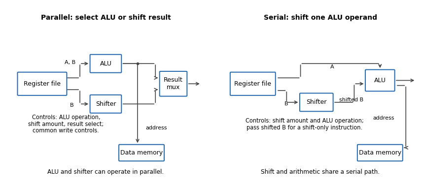
In the parallel design the result-source multiplexer selects either the arithmetic logic unit or barrel shifter. Its control is additional to the ALU function and shift amount. (i) Addition: read the two operands, select ALU addition and select the ALU result; the shift amount is irrelevant. (ii) Constant left bit shift: read the operand to be shifted, set the shift amount from the immediate operand and select the barrel shifter result; the ALU operation is irrelevant.
In the serial design the result comes through the ALU, so that result-source selection disappears. Its shift-amount control is now relevant to arithmetic as well. (i) Addition: set the barrel shifter to zero shift and select ALU addition, so its inputs are the unshifted processor register values. (ii) Constant left bit shift: set the requested shift and select an ALU operation that passes the shifted operand through. If the ALU lacks that operation, implement it or provide a selectable zero on its other input and add zero. This requirement should be stated, rather than assuming that an ordinary two-input add automatically performs a shift alone.
The ALU result can still supply the memory address. For a register-result instruction, enable processor register writeback and leave memory writes disabled. If the ISA requires shift carry flags, the flag-generation control must retain the barrel shifter's outgoing-bit information; blindly using a pass-through ALU's arithmetic carry is insufficient.
Use five cascaded banks of 32 two-input multiplexers, for optional shifts of bits. The original circuit schematic below shows one bank per shift-amount bit; this is a left bit shift with zero fill, not a bit rotation.
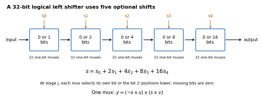


If , stage selects either its unchanged input or that input shifted left by . For bit position , the shifted candidate comes from position when it exists, and otherwise from zero. Composing the chosen stages shifts by the sum of their distances, so each amount from to is represented exactly by its five binary control bits. There are one-bit multiplexers, with five multiplexer delays along a bit path.
A one-bit multiplexer with selector , unselected input and selected input has output . It can be made from one NOT gate, two AND gates and an OR gate; a bank can share the selector inversion. The two possible selector values directly verify its behaviour.
SP-relative addressing forms an effective memory address by adding an offset to the stack pointer. It accesses local variables, saved processor registers or other stack-frame data without dedicating a separate base processor register for each object. The supplied reference gives word-aligned SP-relative offsets from to , which corresponds to an eight-bit nonnegative field scaled by four.
In the modified datapath, select the stack pointer for the unshifted ALU input, the instruction immediate operand for the barrel shifter input, and ALU addition. The effective address can then be . Scaling the immediate operand changes the reachable displacement range without storing a larger immediate operand. For example, an eight-bit field shifted by two reaches offsets through ; shifting it by four reaches through , but only on a sixteen-byte grid. Larger range and finer address granularity are different properties, so the extra reach is not free arbitrary-byte addressing.
The parallel layout cannot feed a shifted immediate operand directly into its address-producing ALU in the same pass. The serial layout can. The actual immediate operand width and permitted shift encodings of a new instruction must be specified; the question does not fix them, so no particular enlarged instruction encoding is implied.
A useful additional mode is base plus scaled register indexing, with effective address . For an array of four-byte elements choose , use its base address on the unshifted ALU input and its index processor register on the barrel shifter input, then add. This forms an indexed machine word address in one datapath pass. An eight-byte element uses .
With parallel ALU and barrel shifter outputs, shifting and adding require either separate instructions/cycles or another route from the barrel shifter to the ALU. The new serial connection supplies that route. This is an addressing mode capability, not a claim that the old instruction encoding already contains the new mode.
The likely effect in a single-cycle or unchanged pipeline-stage implementation is a longer combinational critical path and hence a lower maximum processor clock frequency. Previously the barrel shifter and ALU could work in parallel before result selection; the modified path can require both shift and addition before address or result use.
Ignoring common processor register and wiring delays, the relevant combinational logic contribution changes roughly from to , with any additional input selection included as needed. The processor clock period must also cover processor register timing and the rest of the instruction path, potentially including memory access. Removing a multiplexer offsets some delay, so a numerical frequency change cannot be inferred without component timings. Pipelining, a faster implementation or another pre-existing bottleneck can alter the outcome; the changed serial dependence is the reason for the likely reduction.
For the equal-cardinality basis criterion, because spans , repeatedly remove a vector whenever it is a linear combination of the others. Such a removal does not change the span. The finite process ends with a linearly independent spanning subset , hence a basis of .
If the original were linearly dependent, at least one removal would occur and . But a basis of an -dimensional vector space has vectors. Equivalently, apply the allowed claim to the basis and any fixed -vector basis of : the latter would wrongly be linearly dependent. Thus no removal was possible. The original spanning set is linearly independent and therefore a basis.
Suppose a vector lies outside the span of . Then is linearly independent: in an equation , a nonzero would express in that span, and with the independence of forces every .
This would give linearly independent vectors in a space with an -vector basis, contrary to the supplied claim. Therefore spans . Independence plus spanning makes a basis.
The product is , so multiplying it by the matrix gives an matrix. The product is , so multiplying it on the left by the matrix also gives an matrix. Both multiplications have matching inner dimensions.
For the specified row and column, expand the two matrix products and reorder only finite sums:The middle equality uses scalar associativity and distributivity, and the interchange of two finite sums. Together with their equal dimensions, equality of every entry proves .
Eliminate the first column using multipliers and . The two residual rows have second entries zero and four, so interchange their order for the next pivot. One resulting Pivoted LU decomposition isThe factors below the first pivot must follow the permuted row order, which is why contains before . Direct multiplication gives rows , and in both and . This checks the permutation convention rather than confusing with a different placement of .
Apply the same permutation to the right-hand side and solve two triangular systems. Forward substitution in givesso . Back substitution in gives , , and . Therefore . Substitution in the original system returns , as required.
A triangular matrix has determinant equal to the product of its diagonal entries, so and . A permutation matrix exchanging two rows has determinant . Using multiplicativity of the determinant in yields . Hence .
For nonzero , let be its angle to the unit vector . The scalar projection on the oriented axis is . Since , the dot product identity gives . Multiplying that signed scalar by places the foot at .
The residual is perpendicular to the axis, because . An obtuse angle gives a negative scalar and a foot on the negative side of the line; has projection zero without needing an angle.
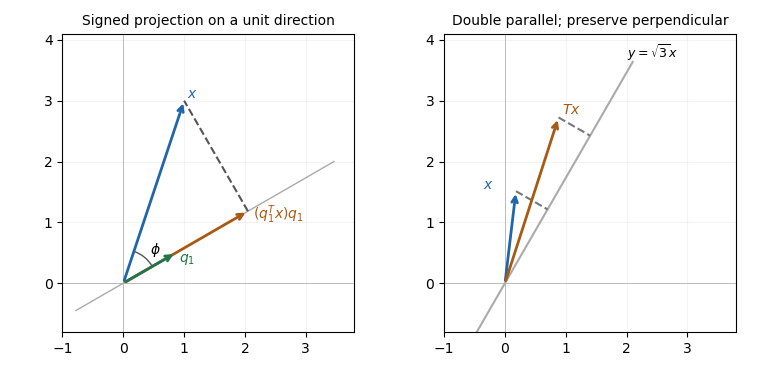
Projection drops a perpendicular to a unit direction; directional stretching doubles only the parallel component
. Details. 
The first panel is a constructed geometric illustration. The second illustrates the directional stretch used later in Question 6.
Consequently for every . Taking successively as the standard basis vectors shows that every column of this difference is zero. Hence . Equality on one selected vector would not suffice; here it holds on all vectors.
Using the unit length of ,Then ordinary matrix expansion gives . Both and its complementary matrix are projectors. The second calculation in fact holds for every idempotent matrix, without requiring the matrix to equal its transpose.
Take . It has exactly two nonzero entries, both one, but . Thus it is not an idempotent matrix. Its being an orthogonal matrix does not make it an orthogonal projector.
Conversely, if , then , which explicitly writes as an image of a linear map under . Hence . The two inclusions prove . No orthogonality assumption was used.
Set . Since , the previous result applies to this projector and gives . Substituting proves . These are the kernel-image identities for complementary projectors.
For a sum of mutually orthogonal projectors, orthonormality gives for and one for . Therefore equals zero for different indices and for equal indices. Expanding the finite sum yieldsThus every stated partial sum is a projector. Its image of a linear map is the span of the first orthonormal set of vectors; arbitrary sums of idempotent matrices would not have this conclusion.
The image of a linear map of is exactly the one-dimensional span of : its formula always returns a multiple of , and . Hence .
The rank-nullity theorem gives . Since by (e)(i), . This includes the case , where the complementary projector is zero.
Update the unknowns in row order, immediately using newly computed components. The component equations areThus and . Using only old values in all three row equations would instead describe the Jacobi method, not the Gauss-Seidel method.
From zero, the first update is . For the next update, the first component is , the second is , and the third is . Therefore .
For the spectral error bound for a diagonalizable fixed-point iteration, the exact solution is a fixed point: . Subtracting it from the iteration gives the error recurrence , with . Multiplying by and using givesIterating proves , including because . This argument does not assume is orthogonal; it simply expresses the error in an eigenbasis.
Write and let . The stated Euclidean norm givesTaking nonnegative square roots proves . At this is equality. This is a contraction bound in the transformed coordinates; an arbitrary nonorthogonal does not give the same unit-constant bound for the original error norm.
The iteration matrix has eigenvalues : expanding its characteristic polynomial down the first column leaves the triangular two-by-two block with diagonal entries . The distinct eigenvalues ensure diagonalizability. Thus its spectral radius is .
The previous bound gives , so the Gauss-Seidel iteration converges for every initial guess under the stated diagonalization. Its limit is the exact solution . Since , a fixed matrix also sends this transformed error to zero; its operator norm can account for any amplification in the original coordinates.
Rotate the specified line onto the horizontal axis, stretch horizontally by two while leaving the orthogonal component unchanged, then rotate back. With and counterclockwise rotation matrix , the requested product isThe rightmost rotation acts first. In particular, and . For the unit direction , the same transformation is . It sends to and fixes every orthogonal vector, verifying that the product is a directional stretch rather than a shear mapping or scaling in every direction. The constructed second panel in the geometric figure in Question 5 illustrates this separation.
Use only the displayed natural deduction rules. Let abbreviate . Indentation below marks temporary assumptions; the closing rule names the assumption discharged.
1  | ¬A                         assume
2  | | φ                        assume
3  | | A                        ∨-intro-L, 2
4  | | ⊥                        ¬-elim, 3 and 1
5  | ¬φ                         ¬-intro, discharge 2–4
6  | A                          ∨-intro-R, 5
7  | ⊥                          ¬-elim, 6 and 1
8  ¬¬A                          ¬-intro, discharge 1–7
9  A                            ¬¬-elim, 8
There are no undischarged assumptions at line 9, so this proves the law of excluded middle. The use of double-negation elimination is explicit; an unproved appeal to the derived RAA rule is unnecessary.
Apply the complete logical derivation of the law of excluded middle in (a) to , obtaining . Then use the disjunction elimination rule, constructing each logical implication by an explicit hypothetical subproof:
1  Q ∨ ¬Q                              result of (a), φ := Q
2  | Q                                 first case
3  | | P                               assume
4  | | Q                               available from 2
5  | P → Q                             →-intro, discharge 3–4
6  | (P → Q) ∨ (P → ¬Q)                ∨-intro-L, 5
7  | ¬Q                                second case
8  | | P                               assume
9  | | ¬Q                              available from 7
10 | P → ¬Q                            →-intro, discharge 8–9
11 | (P → Q) ∨ (P → ¬Q)                ∨-intro-R, 10
12 (P → Q) ∨ (P → ¬Q)                  ∨-elim, 1, cases 2–6 and 7–11
Both case assumptions and both hypothetical assumptions have been discharged. Thus the conclusion is a theorem, not a logical implication that depends on assuming .
Retain the two given logical implications and temporarily assume their common starting proposition.
1  P → Q                    premise
2  Q → R                    premise
3  | P                      assume
4  | Q                      →-elim, 3 and 1
5  | R                      →-elim, 4 and 2
6  P → R                    →-intro, discharge 3–5
Only the original premises remain undischarged, giving the required composition of logical implications.
The logical implication associates to the right. Assume its two antecedents, then use nested applications of the disjunction elimination rule.
1  | P ∨ Q                              assume
2  | | P ∨ ¬Q                           assume
3  | | | P                              first case of 1
4  | | | P                              available from 3
5  | | | Q                              second case of 1
6  | | | | P                            first case of 2
7  | | | | P                            available from 6
8  | | | | ¬Q                           second case of 2
9  | | | | ⊥                            ¬-elim, 5 and 8
10 | | | | P                            ⊥-elim, 9
11 | | | P                              ∨-elim, 2, cases 6–7 and 8–10
12 | | P                                ∨-elim, 1, cases 3–4 and 5–11
13 | (P ∨ ¬Q) → P                       →-intro, discharge 2–12
14 (P ∨ Q) → ((P ∨ ¬Q) → P)             →-intro, discharge 1–13
This proof uses logical falsity elimination rule, but does not need law of excluded middle or double-negation elimination.
For implication creation rule, keep available and discharge an otherwise unused antecedent:
1  ψ                         given
2  | φ                       assume
3  | ψ                       available from 1
4  φ → ψ                     →-intro, discharge 2–3
For implication distribution rule, write . The logical derivation below keeps available and discharges exactly the two temporary assumptions:
1  φ → (ψ → ρ)                          given
2  | φ → ψ                              assume
3  | | φ                                assume
4  | | ψ                                →-elim, 3 and 2
5  | | ψ → ρ                            →-elim, 3 and 1
6  | | ρ                                →-elim, 4 and 5
7  | φ → ρ                              →-intro, discharge 3–6
8  (φ → ψ) → (φ → ρ)                    →-intro, discharge 2–7
These justify both derived inference rules using Figure 2 primitives. Their rule forms retain any other surrounding assumptions; they are not unconditionally asserted conclusions after the displayed numerator is forgotten.
Use the two derived inference rules whose complete proofs were supplied in (d). The following logical derivation has no nested hypothetical subproofs:
1  P → Q                           premise
2  Q → R                           premise
3  P → (Q → R)                     → creation from 2
4  (P → Q) → (P → R)               → distribution from 3
5  P → R                           →-elim, 1 and 4
The creation instance takes and . The distribution instance takes . The metarules are justified in (d); this requested flat use does not secretly invoke implication introduction rule in one of its own lines.
Let abbreviate the given negated existential statement, and choose a fresh variable that is not free in the undischarged premise. Work from an assumed to :
1  ¬∃x (Q(x) → P(x))                  premise N
2  | P(u)                             assume
3  | | Q(u)                           assume
4  | | P(u)                           available from 2
5  | Q(u) → P(u)                      →-intro, discharge 3–4
6  | ∃x (Q(x) → P(x))                 ∃-intro, witness u in 5
7  | ⊥                                ¬-elim, 6 and 1
8  | Q(u)                             ⊥-elim, 7
9  P(u) → Q(u)                        →-intro, discharge 2–8
10 ∀x (P(x) → Q(x))                   ∀-intro, 9, u fresh
The occurrence of in the temporary assumption at line 2 is harmless because that assumption is discharged before universal quantifier introduction rule. No unproved implication-creation rule or quantifier-negation equivalence is needed.
Use the already proved inference in (a) on the negated existential premise. Eliminate the remaining existential with a fresh witness , which must not appear in the final conclusion or the other undischarged assumptions.
1  ∃x P(x)                              premise
2  ¬∃x (Q(x) → P(x))                    premise
3  ∀x (P(x) → Q(x))                     derivation in (a), from 2
4  | P(u)                               fresh-witness assumption for 1
5  | P(u) → Q(u)                        ∀-elim, 3
6  | Q(u)                               →-elim, 4 and 5
7  | P(u) ∧ Q(u)                        ∧-intro, 4 and 6
8  | ∃x (P(x) ∧ Q(x))                   ∃-intro, witness u
9  ∃x (P(x) ∧ Q(x))                     ∃-elim, 1, subproof 4–8
The result in (a) is a proved dependency, not an additional axiom. The witness introduced at line 4 does not escape its subproof.
Assume the existential statement and eliminate it using a fresh witness . Let abbreviate . Instantiating its universal quantification at the witness itself gives two incompatible conditional requirements.
1  | ∃x ∀y ((R(x,y) → ¬R(y,y)) ∧ (¬R(y,y) → R(y,y)))     assume
2  | | ∀y ((R(u,y) → ¬R(y,y)) ∧ (¬R(y,y) → R(y,y)))        fresh witness
3  | | (A → ¬A) ∧ (¬A → A)                                 ∀-elim, 2, y := u
4  | | A → ¬A                                               ∧-elim-L, 3
5  | | ¬A → A                                               ∧-elim-R, 3
6  | | | A                                                  assume
7  | | | ¬A                                                 →-elim, 6 and 4
8  | | | ⊥                                                  ¬-elim, 6 and 7
9  | | ¬A                                                   ¬-intro, discharge 6–8
10 | | A                                                    →-elim, 9 and 5
11 | | ⊥                                                    ¬-elim, 10 and 9
12 | ⊥                                                      ∃-elim, 1, subproof 2–11
13 ¬∃x ∀y ((R(x,y) → ¬R(y,y)) ∧ (¬R(y,y) → R(y,y)))        ¬-intro, discharge 1–12
The contradiction at line 12 contains no free witness variable, so the existential quantifier elimination rule meets its eigenvariable condition. This argument is already valid without classical first-order logic double-negation elimination.
Articles were limited to the first 100 out of 104 total.
Articles by others on the same topic
There are currently no matching articles.