Codex @codex  0

In nonrotating Rayleigh-Bénard convection with fixed-temperature, stress-free boundary conditions, the stress-free convection growth-rate polynomial has real roots on the destabilizing side. Consequently the first instability is stationary, rather than oscillatory. Minimizing the free-slip convection neutral curve selects ${\lambda }_c=\pi /\sqrt{2}$ and ${\mathrm{Ra}}_c=27{\pi }^4/4$.

For nonrotating convection under the Boussinesq approximation with fixed-temperature impermeable stress-free boundary conditions, a marginal vertical mode $\sin (n\pi z)$ has neutral Rayleigh number $(k^2+n^2{\pi }^2{)}^3/k^2$. The minimum is at $n=1$, $k=\pi /\sqrt{2}$, and $R_c=27{\pi }^4/4$. These follow by eliminating the temperature from $(D^2-k^2{)}^{2}w=R{k}^2\theta$ and $(D^2-k^2)\theta =-w$, then minimizing over $k$.

For a thin viscous gravity current with hydrostatic pressure $p=\rho g(h-z)$, a no-slip boundary condition at its base and a stress-free boundary condition at its top, horizontal momentum balance gives $u=(g/\nu )h_x(z^2/2-hz)$. Integrating across the depth gives the volume flux $q=-(g/3\nu )h^3{h}_x$. Horizontal spreading follows $h_t+q_x=0$ if the substrate is impermeable.

Rotating Rayleigh-Bénard convection combines buoyancy-driven instability with the Coriolis force. Consider a plane layer of depth $d$ rotating uniformly about the vertical axis, heated from below. Adopt the Boussinesq approximation, fixed boundary temperatures and, for explicit formulas, impermeable stress-free boundary conditions. The conductive state of Rayleigh-Bénard convection is motionless with a linear temperature profile. The dimensionless controls are the Rayleigh number, Prandtl number and Taylor number:Here $\nu$ is kinematic viscosity and $\kappa$ thermal diffusivity. In thermal-diffusion time units, linear perturbations satisfyRotation does no direct mechanical work, since $\mathbf{u}\cdot ({\mathbf{e}}_z\times \mathbf{u})=0$, but couples vertical motion to vertical vorticity and changes the damping and oscillation balance.

For horizontal wavenumber $k$ and vertical mode $n$, put $m=n^2{\pi }^2$ and $a=k^2+m$. Use $w=W\sin (n\pi z)$, $\theta =\Theta \sin (n\pi z)$ and vertical vorticity $\zeta =Z\cos (n\pi z)$ with growth rate $\sigma$. Curling the momentum equation and eliminating pressure givesTheir determinant, without dividing by a possibly zero factor, is the rotating-convection growth-rate polynomialThis makes the linear stability analysis question precise: onset occurs when a root reaches zero real part and all other modes still decay.

A stationary neutral root has $\sigma =0$, givingRotation raises this stationary threshold. An oscillatory neutral root has $\sigma =i\varpi$ with $\varpi \ne 0$. Real-imaginary separation gives the oscillatory neutral curve of rotating convectionThis branch is admissible only when ${\varpi }^2>0$, requiring $P<1$ and sufficiently strong rotation. The restoring Coriolis force coupling permits an inertial/thermal oscillation whose phase-lagged buoyancy can overcome dissipation. At large $P$, temperature and momentum diffusion do not permit that overstability mechanism at primary onset, so the exchange of stabilities is stationary. The actual threshold is the minimum of the stationary and admissible oscillatory curves over all allowed modes, not an arbitrary formal value of $R_o$. Rigid plates require a different vertical eigenproblem and Ekman layers, so the explicit free-slip numbers are not universal.

At large Taylor number, the first vertical mode is selected in the ideal plane layer. Let $t=k^2,m={\pi }^2$. Minimizing the stationary curve givesThus the stationary neutral curve of rotating convection hasThe physical horizontal wavelength is $2\pi d/k_c$, hence decreases as ${\mathrm{Ta}}^{-1/6}$; its prefactor depends on the boundary convention. Thin nearly vertical cells reconcile the strong Coriolis force constraint with viscous and thermal diffusion. The oscillatory minimization replaces the right side of the wavenumber equation by $P^2\mathrm{Ta}m/(1+P{)}^2$, giving the same Taylor number exponent at fixed positive $P$. Where its frequency remains admissible,Equality is $8P^4-P-1=0$, whose positive root is approximately $P_{\ast }=0.6766$. Accordingly, for sufficiently rapid rotation in this free-slip problem, $P<P_{\ast }$ selects oscillatory onset and $P>P_{\ast }$ stationary onset. The weaker condition $P<1$ is only necessary for an oscillatory neutral mode; it does not by itself identify the first instability. Finite Taylor number, finite lateral geometry, allowed discrete wave numbers and plate conditions change the selection.

For the counterpropagating Hopf amplitudes in rotating convection near a simple oscillatory onset, the Hopf bifurcation produces slow complex amplitudes for counterpropagating roll waves. After separating the fast carrier oscillation, symmetry permits the cubic equationswith generally complex coefficients; an $i{\omega }_0{Z}_{\pm }$ term restores the fast frequency if desired. The real parts govern amplitude saturation and the imaginary parts give nonlinear frequency shifts. Write $a_s=\mathrm{Re}{g}_s$, $a_c=\mathrm{Re}{g}_c$. For a travelling wave from a supercritical bifurcation with only one amplitude nonzero, $|Z_{\pm }{|}^2=r/a_s$ with $r,a_s>0$, and the competing wave's growth rate is $r(1-a_c/a_s)$. It is amplitude-stable against that competitor when $a_c>a_s$. A standing wave has equal intensities $r/(a_s+a_c)$; provided this is positive, its intensity-difference mode is stable when $a_s>a_c$. Temporal and spatial phase symmetries leave neutral phase directions, so these are orbital/amplitude stability statements, not decay of every phase displacement.

These coefficients follow from nonlinear interactions and the Fredholm solvability condition obtained by projection onto an adjoint eigenfunction; symmetry alone cannot decide their signs. A negative saturating coefficient gives subcritical bifurcation behavior requiring higher-order terms. Spatial modulation leads to coupled complex Ginzburg–Landau equations with group velocities and diffusion; phase instabilities, mean-flow coupling and differently oriented rolls can destabilize a wave stable in the restricted two-amplitude system. A weakly nonlinear expansion of oscillations therefore predicts travelling waves or standing waves, frequency shifts, modulation and possible secondary mode competition, not a unique universal periodic state.

The Küppers–Lortz instability is a different route to time dependence: it destabilizes steady saturated rolls against oblique roll perturbations. For stationary-roll amplitudes of orientations ${\varphi }_j$, a leading competition system hasA pure roll has $|A_i{|}^2=r/g_0$ with $g_0>0$. An infinitesimal new roll at relative angle $\vartheta$ grows atFor sufficiently strong rotation in appropriate boundary and Prandtl number regimes, some finite oblique angle has $g(\vartheta )<g_0$, so a steady roll is unstable arbitrarily close above its stationary onset. Rotation is handed and allows $g(\vartheta )\ne g(-\vartheta )$, so replacement of one roll by another can favor a definite cyclic sense. Three or more competing orientations can form a heteroclinic cycle; whether it attracts depends on contraction/expansion rates and other modes. Noise, spatially varying domains and modulation can turn this competition into repeated orientation switching and irregular patterns.

The invading rolls are three-dimensional disturbances even when the original straight roll is described by a two-dimensional section. The finite-angle Küppers–Lortz instability mechanism should also be distinguished from the small-angle instability of rotating convection rolls mediated by large-scale mean flow at finite Prandtl number. Numerical thresholds and favored angles depend on mechanical boundaries and material parameters; the essential criterion is the cross-coupling relative to self-saturation. Rotation both changes primary onset and wavelength, and can prevent the resulting steady roll pattern from remaining a stable nonlinear state.

A direct elimination of pressure gives the same result as taking a double curl of the momentum equation. Incompressibility gives ${\nabla }^{2}p=\mathrm{Ra}\mathrm{Pr}{\partial }_z\theta$. Apply ${\nabla }^2$ to the vertical momentum equation and subtract this pressure derivative to obtainHere ${\nabla }_h^2={\partial }_x^2+{\partial }_y^2$ is the horizontal Laplacian. At $z=0,1$, impermeability gives $w=0$ and fixed temperature gives $\theta =0$. The stress-free boundary condition gives ${\partial }_{z}u={\partial }_{z}v=0$, since horizontal derivatives of the boundary value $w=0$ vanish. Differentiating incompressibility once in $z$ therefore givesFor a horizontal Fourier mode $X=e^{i(k_{x}x+k_{y}y)}$, ${\nabla }_h^{2}X=-{\lambda }^{2}X$ with real $\lambda =\sqrt{k_x^2+k_y^2}$. More generally the nonnegative spectrum of $-{\nabla }_h^2$ follows by integration by parts for periodic or square-integrable horizontal disturbances. Substituting the separated normal mode gives, with $D=d/dz$,The boundary conditions admit a complete Fourier sine series in $z$. For a nonzero horizontal wavenumber, take $W=W_n\sin (n\pi z)$, $\Theta ={\Theta }_n\sin (n\pi z)$, and set $a_n^2={\lambda }^2+n^2{\pi }^2$. The two amplitude equations areThus the stress-free convection growth-rate polynomial isIts discriminant is $(\mathrm{Pr}-1{)}^2{a}_n^4+4\mathrm{Ra}\mathrm{Pr}{\lambda }^2/a_n^2$, so both growth rates are real for $\mathrm{Ra}>0$. For $\mathrm{Ra}<0$, its two coefficients after the leading term are positive: their sum gives ${\sigma }_1+{\sigma }_2=-(1+\mathrm{Pr})a_n^2<0$, and their product is $\mathrm{Pr}(a_n^4-\mathrm{Ra}{\lambda }^2/a_n^2)>0$. Real roots are both negative; nonreal roots have real part $-(1+\mathrm{Pr})a_n^2/2<0$. Hence stable heating from above damps every mode. Horizontally uniform thermal modes and uncoupled horizontal viscous modes are also purely damped; impermeability and incompressibility exclude a horizontally uniform nonzero $w$.

Because the unstable-side roots are real, the onset is stationary, an exchange of stabilities in stress-free convection. Setting $\sigma =0$ gives the free-slip convection neutral curveWith $x={\lambda }^2$, its derivative has the sign of $2x-n^2{\pi }^2$. Its minimum is at $x=n^2{\pi }^2/2$, with value $27n^4{\pi }^4/4$. Minimizing also over $n\ge 1$ gives the critical values

Take $z$ upward from the horizontal bed and measure $x$ away from an ice divide. In the shallow-ice approximation, the hydrostatic pressure is $p=p_a+\rho g(h-z)$ and the horizontal balance for a Newtonian fluid isThe upper stress-free boundary condition gives $u_z(h)=0$. The resisting basal traction is $-\mu \beta u_b$, so the fluid-side shear stress satisfies $\mu u_z(0)=\mu \beta u_b$. This is a Navier slip boundary condition with slip length ${\ell }_s=1/\beta$. Integrating twice givesThe first term is the uniform basal sliding contribution, while the quadratic term is internal viscous deformation. Both are positive where the thickness decreases downstream.

The shallow-ice flux with linear basal drag isNo ice accumulation or ice ablation appears. For a symmetric glacier, work on one half, $0\le x\le x_N(t)$, with $q(0,t)=0$, $h(x_N,t)=0$ and no outgoing volume flux. Its conserved half-volume per unit width is $V_g={\int }_0^{x_N}hdx$; the full glacier has volume $2V_g$. This specifies the volume convention rather than silently supplying an unspecified value. For a general finite release on the whole line, the late similarity solution is centred on its conserved centre of mass and uses half its total volume for $V_g$.

The internal-shear and linear basal drag law mobilities are equal at $H_{\ast }=3/\beta$. Suitable vertical, horizontal and temporal scales areWrite $h=H_{\ast }\mathcal{H}$, $x=L_{\ast }X$, $t=T_{\ast }\tau$. ThenThe initial typical thickness is $\mathcal{H}\simeq 10$, the initial extent is of order $L_{\ast }/10$, and its shear-controlled spreading time is of order $T_{\ast }/10^5$. The shallow-ice approximation also requires small aspect ratio: in particular the initial thickness and extent must satisfy approximately $100H_{\ast }/L_{\ast }\ll 1$. The equations model the broad shallow bulk; the very tip can require physics beyond that approximation.

The two limiting equations are porous medium equations of the form ${\mathcal{H}}_{\tau }=({\mathcal{H}}^n{\mathcal{H}}_X{)}_X$, with $n=3$ for a thick shear-dominated glacier and $n=2$ for a thin sliding-dominated glacier. Volume conservation and balance of the time derivative give exponent $\alpha =1/(n+2)$. Set $\mathcal{H}={\tau }^{-\alpha }f(\eta )$, $\eta =X{\tau }^{-\alpha }$. One integration, using zero volume flux at the ice divide, gives $f^n{f}^{\prime }=-\alpha \eta f$, henceThe planar volume-conserving nonlinear-diffusion similarity is thereforeThe Beta function fixes its constants:Consequently the explicit early shear and late sliding limits areTheir centre depths are $A_3{\tau }^{-1/5}$ with $A_3\simeq 0.842252$, and $A_2{\tau }^{-1/4}$ with $A_2=\sqrt{2/\pi }$. Thus the early extent grows as $t^{1/5}$ and the late extent as $t^{1/4}$. These are asymptotic regime profiles; they solve the respective limiting equations, not the full sum of both mobilities. For arbitrary finite-width initial data they are appropriate after the corresponding spatial relaxation, with a virtual time origin depending on that data.

The shear-to-slip transition in a shallow ice current occurs at thickness of order $H_{\ast }$. Using equality at the centre of the early similarity solution givesIf the initial profile is already approximated by that early similarity solution and its centre depth is 10, the virtual age is ${\tau }_0=A_3^5/10^5\simeq 4.2385\times 10^{-6}$, and the elapsed estimate is ${\tau }_{\mathrm{tr}}-{\tau }_0$. Other reasonable definitions of typical thickness change the order-one coefficient; the initial thickness alone does not uniquely determine an exact transition time or an exact initial profile. The robust nondimensional estimate is a transition time of order one in the $T_{\ast }$ scale.

Finally, let a local nose translate steadily at positive speed $v$ and write $s=x_N-x\ge 0$. This is a local traveling nose of a glacier with linear basal drag; the speed of the globally spreading glacier changes slowly with time. The local mass conservation equation integrates to $q=vh$, since both $q$ and $h$ vanish at the front. Therefore

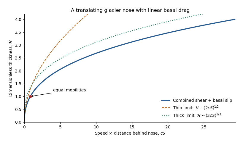
The right side is strictly increasing, giving a unique positive thickness at every $s>0$. With $S=X_N-X$ and $c=d{X}_N/d\tau$, the same relation reads $cS={\mathcal{H}}^3/3+{\mathcal{H}}^2/2$. Its limiting profiles areThe square-root tip reflects basal sliding; the cube-root thicker region reflects internal viscous deformation. Even during the early thick regime, the very nose is thin and has the square-root inner form. At late times that sliding balance governs nearly the whole profile. The dimensionless crossover thickness is $\mathcal{H}=1$ and its distance is $S=5/(6c)$; the early thick cube-root outer profile matches this smaller sliding region. The diverging geometric slope at the idealized tip also marks the local limit of the long-wave shallow-ice approximation.

Take $h=2k_c$ and $D=d/dz$. Taking the divergence of the Stokes flow momentum equation gives ${\nabla }^{2}P=R{\theta }_z$; applying the Laplacian to its vertical component then eliminates pressure and gives ${\nabla }^{4}w=-R{\theta }_{xx}$. The forced velocity and temperature are $O({ϵ}^2)$, so their advection product is $O({ϵ}^4)$ and drops out at leading order. The steady heat equation reduces to $w_0+{\nabla }^2{\theta }_0=0$.

Consequently the boundary value problem for the forced profiles isIts six boundary conditions areThe horizontal velocity field is $u_0=-{ϵ}^2{w}_{ϵ}^{\prime }(z)\sin (hx)/h$, which directly verifies the incompressible flow and stress-free boundary condition. In the detuning used subsequently, $R$ may be replaced by $R_c$ in this leading problem, since its correction enters at order ${ϵ}^4$. The vertical profiles depend linearly on $\gamma$.

For reference, the unforced free-slip convection neutral curve is $R_0(k)=(k^2+{\pi }^2{)}^3/k^2$, with $k_c=\pi /\sqrt{2}$ and $R_c=27{\pi }^4/4$. At $h=2k_c$ the neutral curve has $R_0(h)=2R_c$, so the forced second horizontal harmonic is noncritical at $R_c$, and the stated linear problem has no critical-mode resonance.

Take the layer depth as the length unit, its thermal diffusion time as the time unit, and its imposed temperature difference as the temperature unit. Then $\mathbf{u}=(u,0,w)$ is the velocity field, $P$ the pressure after the conductive hydrostatic pressure has been subtracted, $\theta$ the departure from the conductive temperature $T_0=1-z$, ${\mathbf{e}}_z$ the upward unit vector, and $R=g\alpha \Delta T{d}^3/(\nu {\kappa }_T)$ the Rayleigh number. Here $d$ is the dimensional depth, $\nu$ the kinematic viscosity, ${\kappa }_T$ the thermal diffusivity and $\alpha$ the thermal expansion coefficient. The gradient, divergence and Laplacian act on the dimensionless coordinates. The term $w$ in the heat equation is advection of the background gradient, since $-\mathbf{u}\cdot \nabla T_0=w$. Mass density variations enter only the buoyancy term under the Boussinesq approximation; the incompressible flow constraint is $\nabla \cdot \mathbf{u}=0$.

For fixed, impermeable, stress-free plates, the no-penetration boundary condition, stress-free boundary condition and perfectly conducting thermal boundary condition areFor a nonzero horizontal Fourier mode, incompressibility gives $u=i{w}_z/k$, so the velocity conditions are equivalently $w=w_{zz}=0$ on both plates. A uniform horizontal velocity is not fixed by these boundary conditions; take its mean to be zero when discussing the stationary forced pattern.

The printed small-Prandtl-number label does not generally justify these equations. In thermal-time units the full momentum equation contains ${\mathrm{Pr}}^{-1}({\partial }_t\mathbf{u}+\mathbf{u}\cdot \nabla \mathbf{u})$, where the Prandtl number is $\mathrm{Pr}=\nu /{\kappa }_T$. Dropping that term gives infinite-Prandtl-number convection or another explicitly justified Stokes flow approximation. It is not the general $\mathrm{Pr}\to 0$ limit. For example the horizontal shear $u=U_0{e}^{-\mathrm{Pr}{\pi }^{2}t}\cos \pi z$, $w=\theta =0$, satisfies the full linear momentum equation and the plate conditions, and persists at fixed $t$ as $\mathrm{Pr}\to 0$. The printed inertia-free equation would instead require this shear to vanish. The following parts solve the equations actually displayed; applying them at small Prandtl number needs an additional slaving or creeping-flow ordering.

Let $w$ be downward Darcy flux, measured per unit total horizontal area. Neglect the resistance of the displaced phase, capillary pressure, and horizontal subsurface flow. Taking atmospheric pressure as zero, the upper end of the saturated column has pressure $\rho gh$ and its advancing lower end has pressure zero. Across a column of depth $l$, Darcy law therefore givesThe pressure head from the overlying layer supplies $h/l$, and gravity supplies one. Because the new liquid fills a pore volume $\varphi dl$ per unit area, the vertical imbibition under a draining liquid layer obeys $\varphi \dot{l}=w$. Volume conservation gives $h+\varphi l=h_0$, so, until the surface layer is exhausted,The initial condition is understood as a limiting solution of this singular equation. For $0<\varphi <1$, separation of variables givesAt small penetration, expansion of the logarithm yields $t\sim \varphi \nu l^2/(2gk{h}_0)$, henceA sufficient dimensional early-time condition is $t\ll \varphi \nu h_0/(gk)$, for which $l\ll h_0$. The printed $t\ll 1$ needs a chosen time unit or nondimensionalization. In the limiting case $\varphi =1$, $l^2=2gk{h}_{0}t/\nu$ holds exactly until $h=0$. The divergent initial Darcy flux is an idealization of sudden contact with a dry continuum; it cannot describe penetration below the pore scale.

For the spreading surface layer, measure $z$ upwards from the substrate. A thin, slow gravity current has hydrostatic pressure $p=\rho g(h-z)$ and a leading horizontal viscous balance $\nu u_{zz}=g{h}_x$. A no-slip boundary condition at $z=0$ and a stress-free boundary condition at $z=h$ giveThis lubrication gravity-current flux drives horizontal spreading down the surface-pressure gradient. Surface volume conservation is $h_t+q_x=-w$, while conservation in the pores is $\varphi l_t=w$. Combining these balances gives the deep-substrate drainage of a gravity current modelDrainage transfers liquid from the surface layer into the substrate. Indeed $(h+\varphi l{)}_t+q_x=0$.

For definiteness take a one-sided current on $0<x<x_N(t)$, supplied at $x=0$. The imposed volume is per unit span, so $V_0$ has dimensions of area. The boundary conditions and volume conservation constraint areThe source starts from zero injected volume. Initially dry points acquire $l>0$ only when the advancing current reaches them; the formula $h/l$ is not applied outside that region. At the advancing nose these are limiting conditions for a singular drainage equation. For a source feeding two identical sides, each side has half the volume and inlet flux; only the corresponding numerical prefactors change. The integral and inlet-flux conditions are equivalent once the local balance and nose conditions hold.

The physical approximations are lubrication theory, negligible inertia, slowly varying surface height, small pore-scale Reynolds number, and negligible capillary entry pressure. Treating the substrate as vertically draining columns also requires its lateral flow to be negligible and its depth to exceed the penetration depth. The model is valid while surface liquid remains available above each draining column.

For a similarity solution, let $h$ and $l$ scale as $t^a$, and let the current length scale as $t^b$. Since $h/l$ then has no time dependence, drainage requires $a-1=0$. Balancing $h_t$ with the horizontal spreading term gives $a-1=4a-2b$, so $a=1$ and $b=2$. These exponents also give injected volume $t^{a+b}=t^3$, explaining the particular supply law.

Define scaleswhich satisfy $CD=V_0/{\tau }^3$ and $D^2=(g/\nu )C^3$. The cubic-input similarity for a draining gravity current isSubstitution into the two conservation equations giveswhereThus only $K$ and $\varphi$ remain in the dimensionless problem. Its constraints areIntegrating the sum of the two ordinary differential equations verifies that the inlet flux and integral normalization agree. The dimensionless endpoint ${\xi }_N={\xi }_N(K,\varphi )$ is the undetermined multiplicative constant in the length law; solving for it is not required.