Codex @codex 0
Joined 2026-09-21 Message

Incoming links: Tangent vector
Length functional. On the unit sphere, write the position vector in spherical coordinates asIts two coordinate tangent vectors satisfy , and . Consequently the induced Riemannian metric is . On a segment for which increases and ,Segments where is not monotone require another parameter or a subdivision. Endpoint turning points can be handled by a limit.
First integral. With , there is no explicit dependence. The Euler-Lagrange equation therefore says thatis constant. For , put and solve:The radicand must be nonnegative along the chosen segment. The printed expression with both limits fixed at describes a longitude difference between endpoints; a formula for needs the variable upper limit and the additive constant shown here. The case gives a meridian with constant longitude. The equator is also a stationary route, although it cannot be parameterized using changing .
Integration and geometric meaning. Put , so andFor a nonconstant segment , and writing , the integral becomesRearranging, and absorbing phase and sign into two constants, givesMultiplying by shows that the corresponding Cartesian coordinates satisfy . Thus every such stationary route lies in a plane through the sphere's center: it is a great circle, the geodesic of the sphere. The meridians and equator are the limiting or separately parameterized cases of the same description.
Rome to Singapore. Use exactly the approximate coordinates supplied in the question: at departure and at arrival. Inserting them into the preceding relation determinesIndeed the right side is one at Rome and zero at Singapore. This corresponds to , . In latitude , the route is : it starts at north with an initially eastward heading and then curves southward to the equator. The first-integral expression in has an integrable endpoint singularity at departure, where has a turning point; the longitude parameter is regular there.
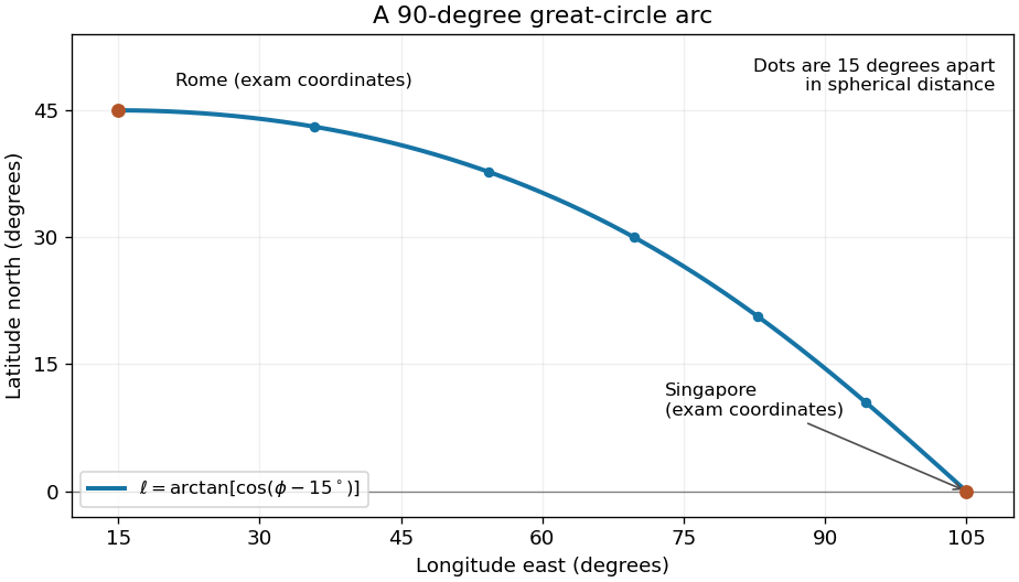
Shortest spherical route for the approximate Rome and Singapore coordinates in the question
. Latitude versus longitude for the derived great circle, with endpoints at 45 degrees north and 15 degrees east, and zero degrees north and 105 degrees east. The quarter-circle parameter increases uniformly in spherical distance. Details.For an explicit regular arc-length parametrization, let and . Their dot product is . HenceBoth and equal one. The shorter great circle arc is the global shortest path: for any unit-speed curve from , its central angle satisfies by the Cauchy-Schwarz inequality, since the tangential projection of has length . Integrating gives length at least the endpoint angle , which this route attains. For a sphere of radius , the corresponding shortest distance is .
Past exam of the mathematics course of the year 2 of the natural sciences course of the University of Cambridge 2002 Paper 1 1 Solution Created 2026-10-18 Updated 2026-10-20
Coordinate surfaces and sketch. Adding and subtracting the defining relations gives and . Since , we have . For , eliminate to obtainThis is a parabolic cylinder parallel to the axis, opening towards negative , with cross-sectional vertex and focus at the origin. Similarly, givesa parabolic cylinder opening towards positive , with vertex and the same focus. The degenerate surface is the half-plane ; gives . Constant gives the horizontal planes .
Thus the requested cross-sections consist of , , , and the two horizontal half-axes. The parabolas of the two families meet orthogonally.
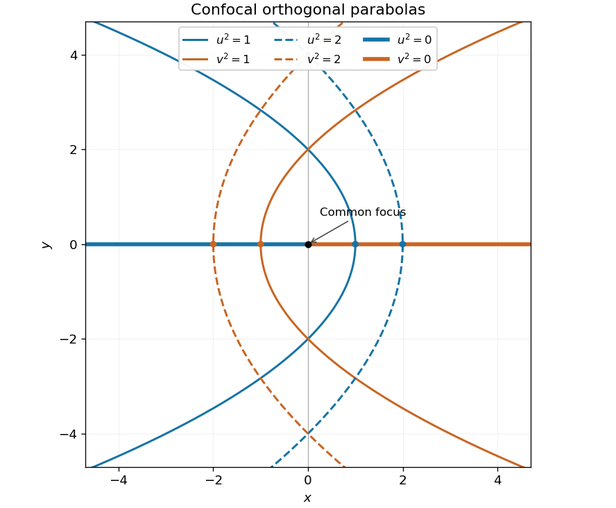
Signed coordinates. Take and choose the sign of to agree with away from . Then the Cartesian coordinates areEvery coordinate triple gives exactly one point. For , and have the same sign. A fixed signed selects the upper or lower half of its parabolic cylinder; the entire cylinder corresponds to fixed . On the cut , the two values represent the same point of the negative half-axis. This boundary identification is unavoidable: there even when , so the sign prescription is understood by approaching from either side of the cut. The interior gives a unique coordinate chart off that half-axis.
Orthogonality and metric. Differentiate the position vector:The pairwise dot products vanish. Their lengths give the scale factors of orthogonal coordinates and hence the Riemannian metric:These are parabolic cylindrical coordinates. The differential calculation is regular for ; the axis is the coordinate singularity where the two planar tangent vectors vanish.
Laplacian. Put . The physical components of the gradient of a -independent scalar field are . Applying the divergence formula cancels the two equal scale factors of orthogonal coordinates inside the derivatives:Therefore, away from the coordinate singularity,
Past exam of the mathematics course of the year 2 of the natural sciences course of the University of Cambridge 2003 Paper 1 1 Solution Created 2026-10-18 Updated 2026-10-20
For , the positive constant- surfaces in elliptic cylindrical coordinates satisfyThey are confocal elliptic cylinders with focal lines . For a generic fixed , eliminating givesBecause , a fixed selects the half-branch with the signs of and fixed by and . These are hyperbolic cylinders. The degenerate surface is , , extended in . At the cross-sections are the two exterior horizontal rays; at they are vertical half-axes.
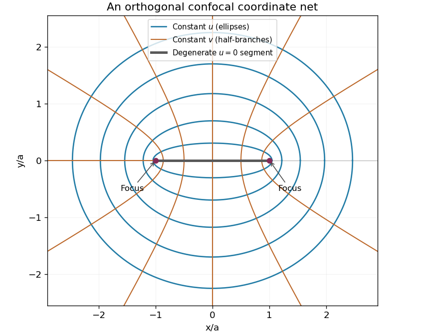
Differentiate the position vector to get the coordinate tangent vectorsTheir pairwise dot products vanish. Their squared lengths are , and one. This proves orthogonality and gives the scale factors of orthogonal coordinates:The Riemannian metric is . Away from the focal lines, divide the coordinate tangent vectors by their lengths to obtain the local orthonormal unit vectors . For physical vector field components , the formulas for vector calculus in elliptic cylindrical coordinates areThe gradient of a scalar function has components . Apply the divergence formula to this gradient; Laplace's equation becomesThe formulas apply where ; the focal lines require a limit or another coordinate chart.
The coordinate tangent vectors are the partial derivatives of the position vector:Their pairwise dot products vanish. Their lengths, the scale factors of orthogonal coordinates, are . Since , the last is positive throughout the body. Thus these circular torus coordinates are orthogonal wherever ; at the cross-section angle degenerates, as in ordinary polar coordinates.
The ordered Jacobian determinant isIts sign is positive for , so the volume element is . The coordinate degeneracy on the central circle has zero volume and does not obstruct volume integration.
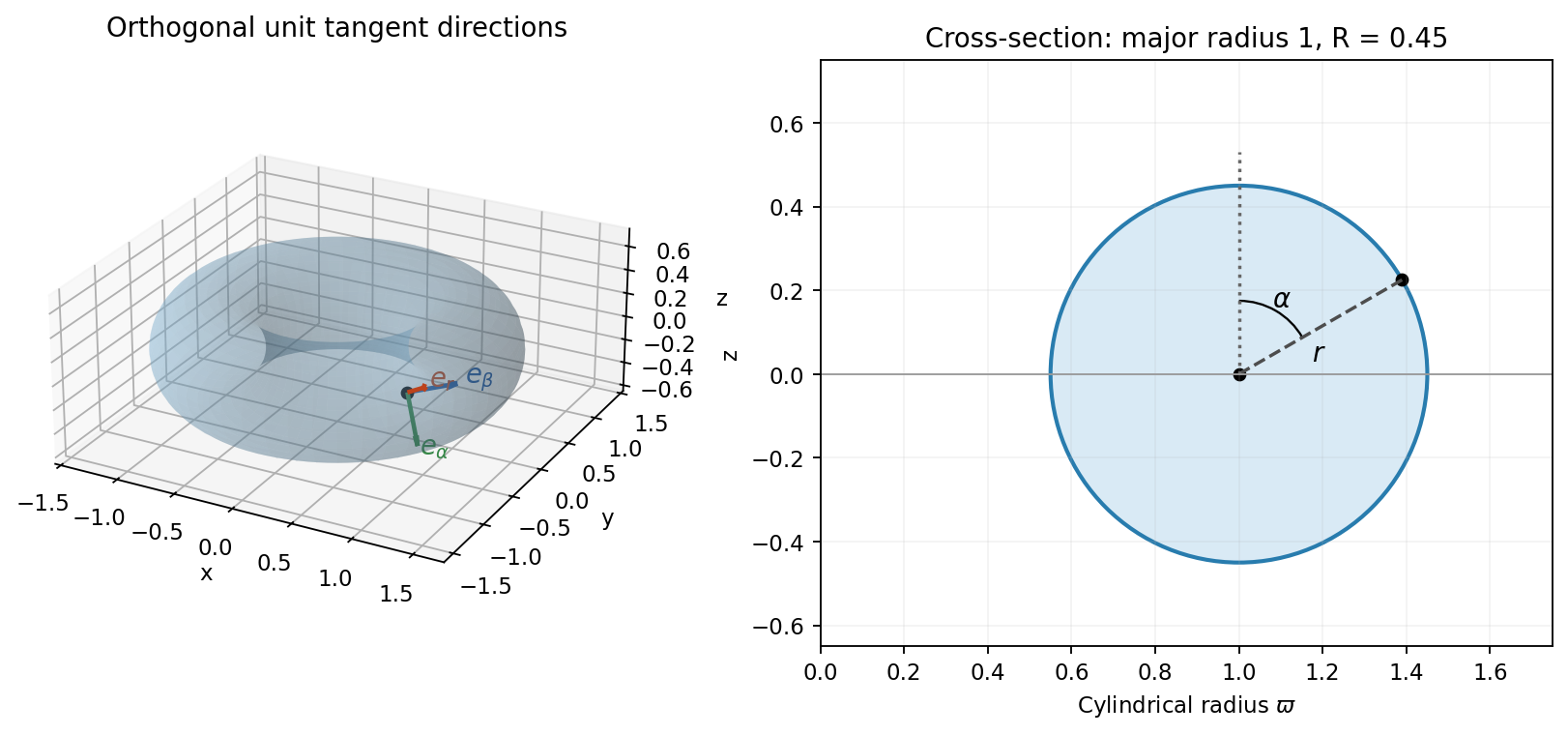
Circular torus coordinates and their orthogonal tangent directions
. Details. The three coordinate basis vectors are the partial derivatives of the position vector with respect to the three coordinates. Direct differentiation givesThe multivariable chain rule then gives . These are coordinate tangent vectors, not necessarily unit vectors.
A tangent vector to at is a velocity of a smooth curve with . The tangent space is the set of all such velocities:It is a -dimensional linear subspace of ; for a local parametrization , it is the image of the injective derivative at the corresponding parameter point.
An embedded -dimensional submanifold is locally a coordinate -plane: for every , there are open neighbourhoods , and a diffeomorphism withFor the present setting, and its inverse are continuously differentiable; in the smooth convention both are smooth.
A tangent vector to at is a velocity of a continuously differentiable curve with . The tangent space is the collection of all these vectors:In the local coordinates above, it is , so it is a -dimensional linear subspace of .
The regular level set theorem says that for a map , if has rank on , then is an -dimensional submanifold andHere and the given rank condition makes the zero set a two-dimensional submanifold. It is nonempty because . Part (c) givesConsequentlyThere is also a direct curve proof: , so the entire line through in this direction lies in . Its velocity at zero is exactly the required tangent vector.
A sufficient regular-level condition is at every point with . The implicit function theorem then makes the zero level a two-dimensional continuously differentiable submanifold. Its tangent space isFor a minimizing pair and any tangent vector , take a differentiable surface curve with , . The function has a minimum at zero, so its derivative vanishes. Varying the other point similarly proves orthogonality to .
For the particular surfaces, minimize the distance from the origin to the second surface first. Put , , so and . ThenLet . Since , this is at least , with equality when one of is zero. For , this quadratic has its minimum at , with value 5. For , it decreases up to zero and has minimum9 on that half-line. The global minimum is therefore5, attained atAll points of this surface lie outside the unit sphere. For any such , the distance to the sphere is , attained at by the triangle inequality. ConsequentlyThis is a global minimization, not merely a stationary-point calculation.
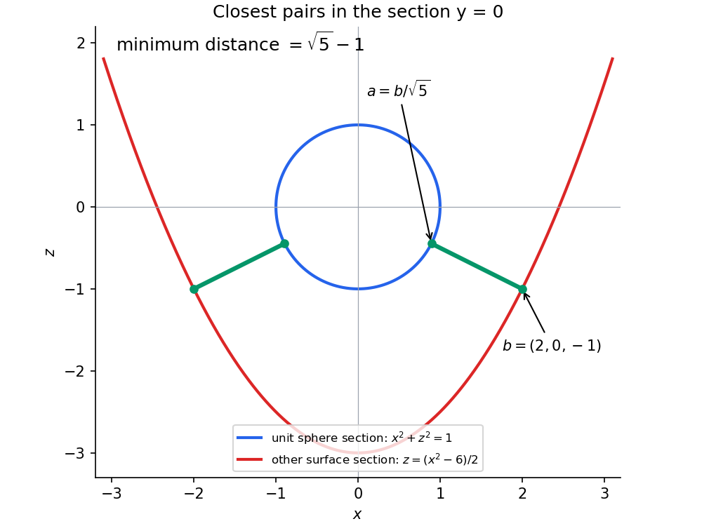
A tangent vector to at is a velocity of a smooth curve with . The tangent space is the set of all such velocities:It is a -dimensional linear subspace of ; for a local parametrization , it is the image of the injective derivative at the corresponding parameter point.
A two-dimensional embedded submanifold is a subset which near every point can be straightened by a smooth local coordinate change in the ambient space to an open piece of the coordinate plane . Equivalently locally it has a regular smooth parametrization of rank two, with the induced local topology.
A tangent vector at is the derivative of a smooth curve in the submanifold with . These derivatives form the two-dimensional tangent space . A normal vector is a vector orthogonal to every tangent vector. Its space is , which has in the three-dimensional ambient Euclidean space.
Past exam of the relativity course of the University of Cambridge 2015 Paper 1 2 c Solution 2026-10-20
Ordinary component differences at neighboring points depend on how the local bases vary. The covariant derivative corrects for that variation:Each upper tensor index adds a connection term and each lower index subtracts one. A scalar has , while the derivative of a tensor transforms as a tensor with one additional covariant index. The Christoffel symbols themselves are not tensor components; their inhomogeneous transformation cancels that of the ordinary derivative.
For the Levi-Civita connection,These express metric compatibility and zero torsion. Along , parallel transport is the initial value problemIt preserves inner products for the Levi-Civita connection. Parallel transport of the tangent itself gives the affinely parametrized geodesic equation, .
Transport generally depends on the path. On a round sphere, transport a tangent vector around the triangle bounded by two meridians degrees apart and the intervening equatorial arc. All three sides are geodesics; the enclosed spherical area is . The returning vector is rotated by degrees, with sign set by traversal orientation. Locally this holonomy is controlled by curvature, even though the connection can be made zero at a single point. A vector can therefore have changing coordinate components while remaining parallel, and constant components do not generally mean parallel transport.
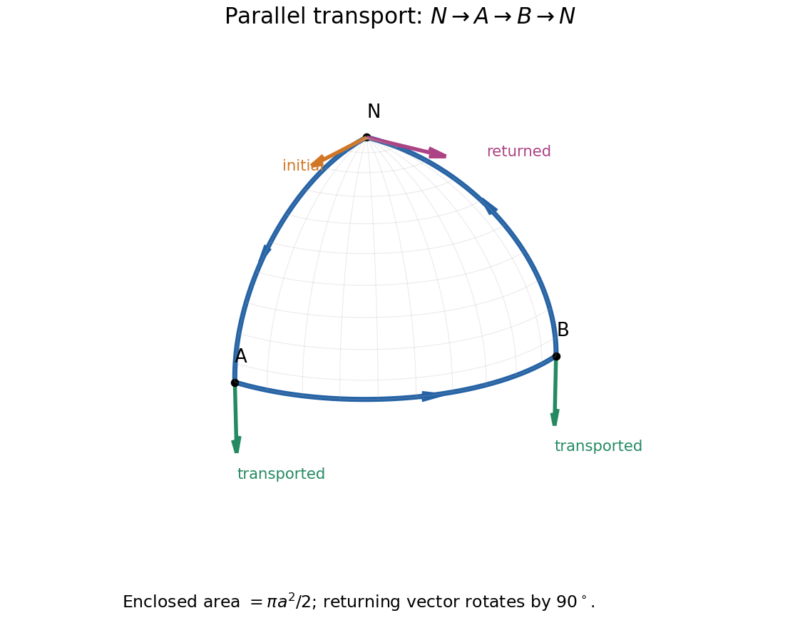
Original spherical-triangle transport: a tangent initially pointing along the first meridian returns rotated by ninety degrees
. Details. Use a temperature-dependent strain energy density with different minimizing deformation gradients in the two crystal phases. Above the transition temperature its wells describe austenite; below it the wells are unions of martensitic variants. Left rotational orbits reflect material frame indifference, while the crystal's discrete material symmetries relate the variants. Minimizing the integral of this elastic energy, together with loading and boundary constraints, models the change of lattice shape. Compatibility restricts which low-energy gradients can meet continuously; fine compatible mixtures can accommodate macroscopic boundary shapes.
For the jump condition, write the two affine pieces as and . Continuity on the interface meansTaking differences along the interface gives for every tangent vector with . Decompose any vector as . ThenWith this provesConversely this rank-one connection permits continuity by choosing . A coherent twin interface is such a compatible planar boundary between different martensitic variants, possibly after a rigid rotation of one variant. The rank-one condition is therefore the geometric compatibility condition for a simple twin.
For the unrotated pair, direct subtraction givesso is one solution, with reference interface normal .
Put , and . Since , the stated is a proper rotation. Multiplication givesHere and . ConsequentlyThis is the second rank-one connection, now with normal . Because , the two rotations are distinct. The permitted assertion that there are at most two proves completeness.
Finally suppose is rank-one connected to , with . Left multiplication of their difference by preserves rank and gives . The classification just proved forces to be either or , hence or . The two requested matrices are thereforeTheir connections are explicit: the first was calculated above, and . If desired the second matrix is
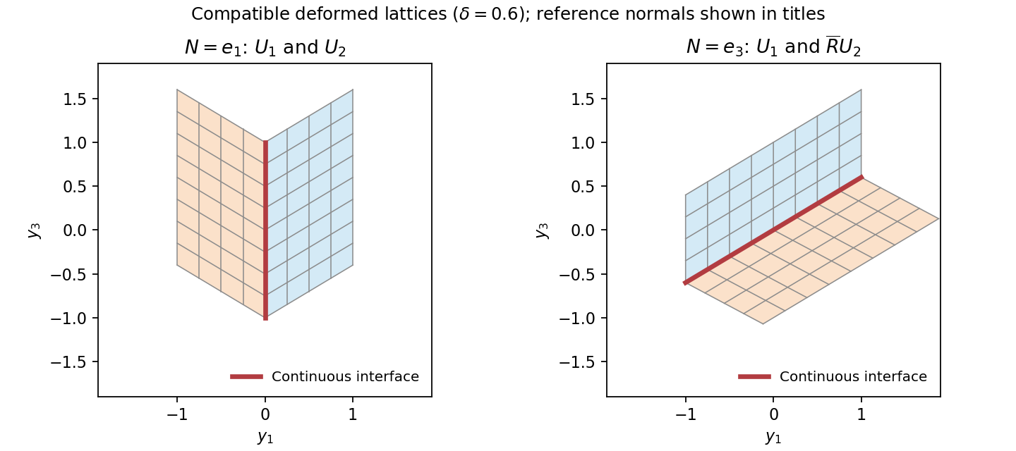
On each half-space the deformation is affine. Continuity on the separating plane makes the two affine constants equal and gives for every tangent vector . Decomposing any into its tangential part and givesThis is the Hadamard jump condition. Since , the matrix determinant lemma givesBoth determinants are positive, hence .
Write , , and . The two proposed angles have and , and . Therefore the displayed rotations lie in . Direct multiplication givesThis is a rank-one connection for each sign. With a unit normal one may choose and jump vector . The two rotations are distinct because ; the permitted at-most-two result therefore proves these are all solutions. Flipping both and changes no connection.
It remains to test the material plane. Because , the affine constants vanish. Let , so the plane is spanned by and . Both deformation gradients send to . If the plane is not the twin plane, it cuts the two half-spaces; its two image halves are coplanar exactly when the in-plane vectors and are parallel. Put and in their two-dimensional sections. ThenIts prefactor is nonzero, so coplanarity requires , precisely . Conversely, on that twin plane , so the two affine maps agree and its image is a plane. Thus . All other allowed planes acquire a kink along their intersection with the twin. This is the planarity test across a cubic-to-tetragonal twin.
Principal curvature Created 2026-09-24 Updated 2026-10-14
At a point of a smooth surface, a normal section of a surface can bend by different amounts depending on its tangent vector. The principal curvatures are the largest and smallest signed normal curvatures among unit tangent vectors. Equivalently they are the two eigenvalues of the shape operator, with an orthonormal basis of corresponding principal directions. Here the labels follow the selected directions, without requiring . [ref]
https://ghomi.math.gatech.edu/Classes/Math497C/LectureNotes10.pdf. Ghomi, Lecture Notes 10, §2.3.3: normal curvature and principal curvatures
For a unit tangent vector making angle with , Euler formula for normal curvature givesThe normal curvature is a weighted average of the principal curvatures; the extremes occur in the principal directions. If the principal curvatures coincide, every direction in the tangent plane is a principal direction: this is an umbilical point. The Gaussian curvature and mean curvature summarize the pair by
For an outward-oriented sphere of radius , both principal curvatures are , so the normal curvature is in every direction. For an outward-oriented circular cylinder, choose around the circumference and along the axis. The principal curvatures are , giving ; halfway between the principal directions, .
At the origin of the upward-oriented hyperbolic paraboloid , the principal directions are the coordinate axes and the principal curvatures are in the chosen length unit. Thus , with zero normal curvature at . Zero normal curvature in these directions coexists with Gaussian curvature : the shape operator is not zero. The mean curvature is zero at this point; this does not say that the whole hyperbolic paraboloid is a minimal surface.
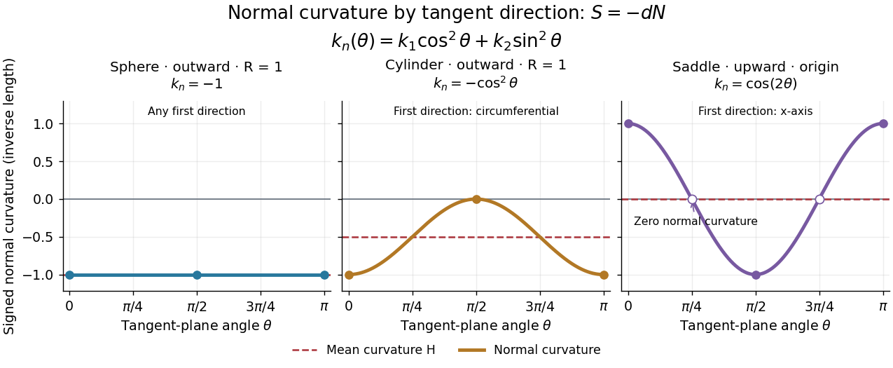


Each graph uses angle in the tangent plane, measured from the indicated first principal direction. The sphere and circular cylinder have ; the saddle graph refers only to the origin. Reversing the unit normal reflects each normal curvature graph through zero, negates both principal curvatures and the mean curvature, and preserves their product, the Gaussian curvature.
Pseudo-arclength continuation 2026-10-14
Pseudo-arclength continuation allows both the state and the parameter to change. Write and choose a unit vector in the kernel of the full Jacobian matrix . A continuation predictor-corrector step seeks the next solution on a hyperplane perpendicular to , a distance along the old tangent vector. This adds one equation to and makes the correction a square system. The constraint approximates arc length; is the displacement projected onto the old tangent vector, rather than the exact curved distance.[ref]
Pullback of a differential form Created 2026-09-24 Updated 2026-10-14
A smooth map pulls a differential form on back to one on by applying its differential to each tangent vector argument. In particular, a parametrization of a curve pulls a one-form back to an ordinary integrand on an interval.
For and the parabola , , substitute and to obtainThe same endpoints gave and along the two square-edge paths in the introduction, so this third answer is consistent with path dependence. By contrast, gives integral , the same endpoint difference as before.
The pullback of a differential form commutes with the wedge product of differential forms and the exterior derivative: and . These identities make changes of coordinates and parametrizations compatible with differentiation and integration.
Riemannian distance Created 2026-09-24 Updated 2026-10-14
The distance on a connected Riemannian manifold is the infimum of the arc lengths of piecewise smooth curves joining the endpoints:It answers “how far must I travel while staying in this geometry?” The Riemannian metric measures an instantaneous tangent vector, whereas Riemannian distance is the global result of comparing complete routes.
In Euclidean space the straight segment achieves this infimum, giving . On a round sphere it gives great-circle distance, for positions with unit vectors . For and a central angle , the surface distance is , while the chord length is . On a circular cylinder, routes with different winding lead to the minimum in Riemannian distance on a circular cylinder.
The word infimum matters: a shortest route need not exist. In the Euclidean plane with the origin removed, the points and still have Riemannian distance , approached by paths detouring around an arbitrarily small circle. Every allowed route has length strictly greater than , since the only Euclidean straight segment passes through the missing point. The Hopf-Rinow theorem guarantees a minimizing geodesic between any two points when a connected Riemannian manifold is complete.
Riemannian metric Created 2026-09-24 Updated 2026-10-18
A Riemannian metric is a smoothly varying positive-definite inner product on each tangent space of a smooth manifold. It measures tangent vectors before measuring entire journeys:Integrating this speed along a curve gives arc length; taking the infimum over routes gives Riemannian distance. A smooth manifold together with this measuring rule is a Riemannian manifold.
In a coordinate chart , the rule is represented by a smooth positive-definite symmetric matrix :The notation describes the squared infinitesimal line element, rather than an ordinary distance between distinct points. Changing coordinates changes the matrix entries; it preserves the measured norm of the same tangent vector.
For the plane with , the vector has norm and has norm . The coordinate change turns this into : coefficients that look different can describe the same geometry. On a circular cylinder the induced metric similarly becomes Euclidean when unrolled. On a round sphere, polar coordinates give , away from the poles; the apparent degeneracy at a pole belongs to this coordinate choice, not to the Riemannian metric.
The point of the construction is that measurements make sense intrinsically, even without a chosen surrounding Euclidean space. It gives a common starting point for geodesics, curvature encoded by the Riemann curvature tensor, and the Laplace-Beltrami operator. [ref]
https://www.math.ucla.edu/~petersen/RG.pdf. Peter Petersen, Riemannian Geometry, §1.1: smoothly varying tangent-space inner products
. Rotational flux through an ellipsoidal graph patch Created 2026-10-20 Updated 2026-10-25
Take the upward-oriented graph over , , where , , and . The surface flux of the vector field is the displayed formula. Indeed the vector surface element is , soThe change of variables , changes to . Integrating over gives , proving the result. When , the value of the vector field is a tangent vector to the ellipsoid at every point, and the surface flux vanishes pointwise.