Codex @codex  0

Absolute thermodynamic temperature can be defined so that a reversible engine exchanging heats $Q_h$ and $Q_c$ with reservoirs at $T_h$ and $T_c$ satisfiesA choice of one reference temperature fixes the scale.

Thermoelasticity couples elasticity and temperature through a specific Helmholtz free energy $\psi (F,\theta )$. Without constraints its reversible laws are $P_{Ii}={\rho }_0{\psi }_{,F_{iI}}$ and $\eta =-{\psi }_{,\theta }$. Mixed derivatives give the same coupling tensor in the thermal stress response and the strain dependence of specific entropy, with opposite signs.

The chosen steady-state model isHere $U$ is the terminal voltage drop along positive electric current through the module. Its Seebeck effect term opposes the cooling supply. The cold Peltier effect term removes heat; Joule heating and returning heat conduction reduce the available cooling. At zero electric current, $Q_c=Q_h=-K\Delta T$: the passive leak warms c and removes heat from h, consistent with the stated signs. Subtracting the two face equations cancels heat conduction and gives the electrical power, an independent conservation of energy check.

The factor one half is an ideal-model result, not a universal rule for every contact. To see its origin, let $x$ run from cold to hot along a uniform equivalent leg of length $L$, cross-sectional area $A$, electrical resistivity $\rho$ and thermal conductivity $\kappa$. With constant coefficients, insulated sides and no Thomson effect, steady conservation of energy givesThe Fourier's law heat current in the positive $x$ direction is $-\kappa A{T}^{\prime }$. At $x=0$ it equals $-K\Delta T-I^{2}R/2$, and at $x=L$ it equals $-K\Delta T+I^{2}R/2$, using $K=\kappa A/L$ and $R=\rho L/A$. Adding the local transported heat current $\alpha TI$ gives the two face equations. Summing equivalent legs preserves this accounting. Nonuniform material properties, side losses or asymmetric contact dissipation require a revised model.

For an original toy module, stipulate $\alpha =0.040V/K$, $R=2.0\Omega$, $K=0.40W/K$, $T_c=280\mathrm{K}$ and $T_h=300\mathrm{K}$. At $I=3.0\mathrm{A}$,The coefficient of performance is defined here only for refrigeration with $Q_c>0$ and $P_{\mathrm{in}}>0$. The hot-side assembly must remove $37.0\mathrm{W}$, not just the extracted $16.6\mathrm{W}$. These are stipulated calculations, not measurements or a commercial module specification.

At the same fixed face temperatures but $I=-3.0\mathrm{A}$, the same boundary definitions give $Q_c=-50.6\mathrm{W}$, $Q_h=-35.0\mathrm{W}$, $U=-5.2\mathrm{V}$ and $P_{\mathrm{in}}=15.6\mathrm{W}$. The formerly cold face is now heated; the formerly hot reservoir supplies $35.0\mathrm{W}$. Still $Q_h-Q_c=15.6\mathrm{W}$. Reversal changes the linear terms, while $I^{2}R$ and the leak at fixed temperatures remain unchanged. Holding the old labels fixed makes this check meaningful.

The corresponding steady entropy production of the module is the outgoing reservoir entropy minus the incoming reservoir entropy:The Peltier effect terms cancel because they carry the same entropy $\alpha I$ at each end. This cancellation explains the reversible coupling; it does not make finite-resistance operation reversible. In the toy example the two positive contributions are approximately $0.06214$ and $0.001905W/K$, giving ${\dot{S}}_{\mathrm{gen}}=0.06405W/K$ for either current direction. In cooling operation, combining this inequality with the energy balance gives the Carnot refrigerator limit $\mathrm{COP}\le T_c/(T_h-T_c)$, equal to $14$ for these reservoir temperatures. A coefficient of performance above one would describe transported heat per electrical work, not the creation of energy.

Thermoelectric cooling uses the Peltier effect to remove heat from a load using electrical work. A typical thermoelectric module connects many pairs of different semiconductors electrically in a series circuit and thermally in parallel between two faces. For an idealized pair with $S_p>S_n$, positive conventional current crosses n to p at the cold bridge and p to n at the hot return. With common bridge material and isothermal contacts, the intervening metal contributions telescope: the net pair coefficient is $S_p-S_n$. For $N$ identical pairs define the module Seebeck coefficient $\alpha =N(S_p-S_n)>0$.

Choose fixed face temperatures $T_h\ge T_c>0$, $\Delta T=T_h-T_c$, module electrical resistance $R>0$ and open-circuit thermal conductance $K>0$. All three module parameters $\alpha ,R,K$ are constants over the chosen operating range. Positive $I$ is the orientation absorbing Peltier effect heat at c. Define $Q_c$ as net heat extracted from the cold reservoir per unit time, $Q_h$ as net heat delivered to the hot reservoir per unit time, and $P_{\mathrm{in}}$ as electrical power entering the module. Despite the conventional letters $Q_c,Q_h$, both denote power in watts, not accumulated energy. Ferrotec gives the corresponding single-stage equations and distinguishes module performance from bypass leaks.^[ref]

At fixed face temperatures, differentiation of the thermoelectric cooler energy balance givesThus current chosen for maximum cooling power is not automatically current for maximum coefficient of performance. Cooling exists only when $(\alpha T_c{)}^2>2RK\Delta T$, and then only between the two positive rootsAt equality the parabola merely touches $Q_c=0$. For the toy module the interval is approximately $0.767<I<10.433\mathrm{A}$, with $I_{\ast }=5.60\mathrm{A}$ and $Q_{c,\max }=23.36\mathrm{W}$. At $12\mathrm{A}$, the object is heated even in the nominal cooling polarity: $Q_c=-17.6\mathrm{W}$. This mathematical interval supplies no permission to exceed an actual device's current or temperature ratings.

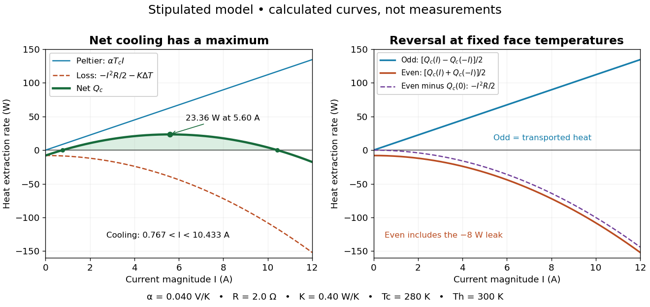
The fixed-face constraint matters. With fixed $T_h$ but a freely cooling object, $T_c$ must be solved from its heat load and leaks rather than held at $280\mathrm{K}$ while claiming an arbitrary temperature drop. For zero load and optimal current, the same model givesHere $Z$ has units ${\mathrm{K}}^{-1}$ and is a module parameter. The toy model gives $Z=0.0020{\mathrm{K}}^{-1}$ and $T_{c,\min }\approx 241.62\mathrm{K}$ when $T_h=300\mathrm{K}$. This is an ideal zero-load limit with stipulated constant properties; cooling a real load requires $Q_c$ above zero and reduces the attainable drop. Contact thermal resistance, a warming heat sink, external leaks and temperature-dependent coefficients further change the result. Electrical control is convenient, but conservation of energy still requires a thermal path that removes the extracted heat plus the electrical input.

For a constant-property pair with Seebeck difference ${\alpha }_{np}$, electrical resistance $R$ and thermal conductance $K$, $Z_{\mathrm{pair}}={\alpha }_{np}^2/(RK)$. With identical legs of individual resistivity $\rho$ and thermal conductivity $\kappa$, this is ${\alpha }_{np}^2/(4\rho \kappa )$, not ${\alpha }_{np}^2/(\rho \kappa )$.

A thermoelectric effect couples heat transfer and the transport of electric charge: a temperature gradient can generate an electromotive force, while an electric current can carry heat and cause heating or cooling at a junction of different materials. This coupling makes electrical measurement of temperature possible through a thermocouple, and permits conversion of a sustained flow of heat into electrical work. A finite open-circuit voltage does not itself deliver power: electrical power requires an electric current through a load. Thermoelectric conversion therefore involves both electromagnetism and thermodynamics. ^[ref].

The dimensionless material figure of merit is $ZT=S^2\sigma T/({\kappa }_e+{\kappa }_l)$. Device efficiency depends on its temperature dependence and parasitic losses, not only on one peak value.

A generator using the Seebeck effect to convert a temperature difference into electrical output.

The combination $S^2\sigma$ of Seebeck coefficient and electrical conductivity. Increasing it alone need not increase ZT if thermal conductivity rises as well.

The thermomechanical effect couples a temperature difference to a pressure difference across a superleak. For the closed-chamber model in the apparatus figure, consider neighboring equilibrium states with small velocities, negligible height difference and pure helium-4. Let ${\mu }_m$ be chemical potential per unit mass, in $\mathrm{J}\mathrm{k}{\mathrm{g}}^{-1}$. The Gibbs free energy differential per unit mass givesThe superleak allows the superfluid to redistribute until the two sides have equal ${\mu }_m$. Setting $d{\mu }_m=0$ therefore givesThe sign matters: heating one side at initially equal pressure lowers its ${\mu }_m$; inflow raises its pressure until chemical balance is restored. The hotter side has the higher pressure. The integral follows the constant-${\mu }_m$ path; it need not be evaluated at fixed pressure when material properties vary appreciably.

For an original local example, stipulate constant $\rho =150\mathrm{kg}{\mathrm{m}}^{-3}$, $s=100\mathrm{J}\mathrm{k}{\mathrm{g}}^{-1}{\mathrm{K}}^{-1}$ and $T_h-T_c=0.020\mathrm{K}$. The predicted pressure difference is $300\mathrm{Pa}$. These are teaching assumptions, not helium measurements. This static thermodynamics relation predicts neither the required heater power nor the filling time: those require heat leakage, channel conductance and chamber heat capacity. An outlet would introduce kinetic energy and a flowing balance, so the static $300\mathrm{Pa}$ is not a predicted fountain height.

A thermometer measures temperature through a physical response whose relation to temperature is known. Examples include the length change from thermal expansion, a change in electrical resistance, and the pressure of a gas thermometer. If the response function $X=f(T)$ is an injective function over the working range, its measured value determines $T=f^{-1}(X)$ through the inverse function. Thermometer calibration establishes that relation for the particular instrument and measurement conditions. Two matching readings are meaningful only after calibration to a common scale and with the probes sampling comparable equilibrium states. ^[ref]

For a contact thermometer, the sensing part must reach thermal equilibrium with the region being measured. That region may differ from the rest of the object: an immersed probe near a heater can read a local temperature while the surrounding water remains cooler. A stable reading can also be a steady state set by competing heat transfer paths to the sample and the room. Good contact, adequate immersion, mixing where appropriate, and checks for spatial differences help establish which temperature the reading represents. These are measurement controls inferred from the thermal equilibrium requirement, not a guarantee that every flat trace is equilibrium.

A thermometer also changes the sample it touches. Consider an original toy calculation with an initially uniform sample at $T_o=350\mathrm{K}$, a probe at $T_p=300\mathrm{K}$, and constant whole-body heat capacities $C_o=100\mathrm{J}{\mathrm{K}}^{-1}$ and $C_p=1\mathrm{J}{\mathrm{K}}^{-1}$. Suppose together they form an isolated system, with no work or phase transition and negligible contact energy. The first law of thermodynamics and thermal equilibrium giveThe final thermometer reading underestimates the sample's original temperature by about $0.495\mathrm{K}$, although it correctly measures their new common temperature. The disturbance becomes small when the participating probe heat capacity is small compared with the sample's. A large controlled heat bath is a different limit: it supplies or removes heat while approximately maintaining its own temperature.

Waiting time is a separate issue from disturbance. Under a toy Newton's law of cooling model for a uniform probe in a maintained heat bath, a constant contact conductance $G$ givesThe time constant $\tau$ controls this exponential decay. For stipulated values $T_b=350\mathrm{K}$, $T_p(0)=300\mathrm{K}$ and $\tau =5\mathrm{s}$, the probe reads about $331.61\mathrm{K}$ after one time constant and $347.51\mathrm{K}$ after three. These are calculated values, not an instrument specification or measured data. Real probes may have multiple relaxation times and additional heat transfer paths; choose an equilibration criterion from the required accuracy, rather than assuming that a fixed waiting time works universally.

Thermometer calibration compares an instrument's response with assigned reference temperatures under specified conditions. In a proposed two-reference procedure, thermalize the sensing part at $T_0$ and $T_1$, record responses $X_0$ and $X_1$, and, only if a linear response is justified over that interval, useAdditional reference temperatures test curvature; returning to the first reference tests drift. A gas thermometer instead obtains its response from an equation of state, with a reference and corrections for its apparatus. In either case, uncertainty in the reference propagates to the inferred temperature. Calibration determines the response relation; it cannot by itself remove the finite-sample disturbance or incomplete thermal equilibrium described in thermometer. A reference established on a practical scale can also differ slightly from true thermodynamic temperature; the BIPM distinguishes the International Temperature Scale of 1990 readings from their thermodynamic counterparts.^[ref]

A thermopile connects multiple thermocouples in series to turn a temperature difference into a larger electrical signal. Absorbed thermal radiation can heat its sensing junctions while reference junctions remain cooler; the signal depends on the thermal and optical design.

A thermopile is an array of thermocouples connected as a series circuit with their electromotive forces adding in the chosen terminal order. It measures a collective temperature difference through the Seebeck effect. An open-circuit electric potential difference requires no externally supplied electric current through the array: a high-input-electrical resistance voltmeter reads the signal. The heat that maintains the junction temperature difference still comes from somewhere, such as absorbed electromagnetic radiation.

In a membrane detector, an absorbing film heats the measuring junctions while reference junctions lie on the surrounding support. Actual junction temperatures can differ across the membrane.^[ref] This converts difficult-to-observe heat transfer into an accessible electrical signal; the series connection combines many small contributions without requiring every thermocouple to have a separate meter.

A thermopile absorber converts incident electromagnetic radiation into heat near the thermocouple measuring junctions. Electrically separate junctions can share its temperature through thermal contact. The reference support provides a path for heat transfer and a comparison temperature; “cold” denotes this reference role, even if it is warmer than the absorber.

Distinguish incident power from absorbed power. A window, the illuminated area, and the absorption of the coating determine their relation. A detector's measured voltage sensitivity can depend on where a small illuminated spot lies.^[ref] The model in thermopile thermal response takes absorbed power as its input, so an optical calibration is a separate step.

PASCO's documented lamp experiment connects a TD-8553 thermopile sensor to a millivoltmeter and places it level with a lamp filament along a meter stick. Lamp and detector axes are aligned. With the lamp off, readings at several positions establish an average ambient thermal radiation background. With the lamp on at a fixed supply setting, detector readings at different distances are compared after background subtraction. Between readings, a reflective shield prevents the detector warming; its shutter also protects the reference junction when idle. Moving the shutter can move the sensor, so fixed geometry matters. The manual's lamp limits must be followed.^[ref]

This protocol tests whether the background-corrected electric potential difference approximately follows the inverse-square law over a suitable distance range. It is a relative electromagnetic radiation measurement; those readings alone do not calibrate absorbed power in watts. The manual treats the filament as an approximate point source.^[ref]

For an absolute calibration, independently known absorbed power and a monitored reference temperature would be needed. A useful additional control is to repeat a fixed detector position before and after a distance sweep: disagreement reveals possible drift. These additions test the measurement chain rather than assuming that background subtraction fixes every error. A finite source, changing illuminated area, reflections, changing reference temperature, and insufficient settling can alter the measured dependence. In particular, the time constant in thermopile thermal response explains why a quick reading and a settled reading may differ. The detector infers its own absorber temperature difference; inferring the source's temperature additionally requires its emissivity, optical geometry and an appropriate thermal radiation model.

Use the A-positive terminal order of Seebeck effect for each thermocouple. Its thermocouple measuring junction has temperature $T_{h,i}$ and its reference connections have temperature $T_{c,i}$. Define the difference of Seebeck coefficients as ${\alpha }_i(T)=S_{A,i}(T)-S_{B,i}(T)$. Connect the B reference end of one thermocouple to the A reference end of the next at a common local temperature, so the terminal electric potential differences add:The first A reference terminal is the positive meter input; the final B reference terminal is the negative input. Following this connected path and adding the individual Seebeck effect integrals proves the result. Matched meter leads with common endpoint temperatures cancel as in an isothermal terminal block. The manufacturer's sum formula also allows unequal individual contributions.^[ref]

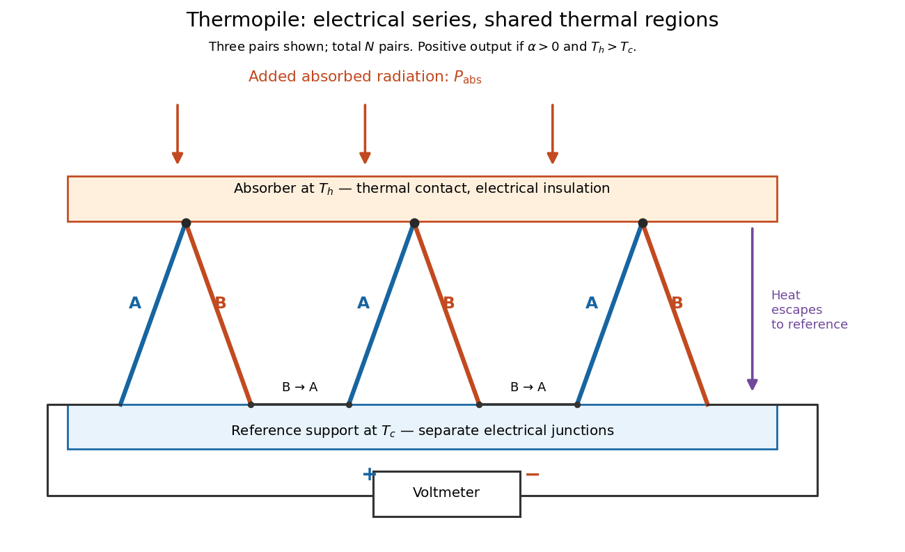
If all pairs share $T_h,T_c$ and the same nearly constant difference $\alpha$ of Seebeck coefficients throughout that temperature interval, thenThis $\alpha$ is the pair's relative Seebeck coefficient, not either material's individual coefficient or a universal device constant. As an original constructed example, choose $N=20$, $\alpha =40\mu \mathrm{V}{\mathrm{K}}^{-1}$ and $\Delta T=5\mathrm{K}$. Each thermocouple contributes $0.20\mathrm{mV}$ andReversing the meter connections changes the sign. Exchanging $T_h$ and $T_c$ reverses the integrals and hence the electromotive force; this reversible sign response does not make a detector with heat conduction a reversible thermodynamic process. Reversing the wiring of one pair instead gives $(N-2)\alpha \Delta T$, because one contribution is subtracted rather than added. For this example the result is $3.6\mathrm{mV}$, and at equal junction temperatures every contribution vanishes.

The open-circuit condition matters. If the array's total electrical resistance is $R_{\mathrm{pile}}$ and the meter input has electrical resistance $R_m$, the elementary voltage divider model gives $V_m=V_{\mathrm{oc}}{R}_m/(R_m+R_{\mathrm{pile}})$. Thus $R_m\gg R_{\mathrm{pile}}$ is needed to suppress voltmeter loading. Appreciable electric current also permits Joule heating and the thermoelectric heat transfer to disturb the assumed junction temperatures.

A useful original model treats the thermopile absorber as one approximately uniform temperature $T_h(t)$ with heat capacity $C_{\mathrm{th}}$, connected to a fixed reference temperature $T_c$ by thermal conductance $G_{\mathrm{th}}$. Both parameters are positive constants here. Let $P_{\mathrm{abs}}(t)$ be an added absorbed power above the initial background. Linearize the outgoing heat transfer about that background. With $\Delta T=T_h-T_c$ measured from an initial state having $\Delta T=0$, conservation of energy gives the first-order linear differential equationThe left side is the rate of stored energy; the two terms on the right are added power and outgoing heat transfer. The effective thermal conductance can include several paths, rather than just heat conduction along the wires. The model assumes a stable reference, negligible electrical loading, a common absorber temperature, and changes small enough for constant parameters.

For a step from zero to constant $P_0$ at $t=0$, subtract the steady solution $\Delta T_{\infty }=P_0/G_{\mathrm{th}}$. The difference obeys exponential decay, so the initial condition fixesThe time constant has units $(\mathrm{J}{\mathrm{K}}^{-1})/(\mathrm{W}{\mathrm{K}}^{-1})=\mathrm{s}$. With the same constructed $N=20$ and $\alpha =40\mu \mathrm{V}{\mathrm{K}}^{-1}$, choose $C_{\mathrm{th}}=0.02\mathrm{J}{\mathrm{K}}^{-1}$, $G_{\mathrm{th}}=0.01\mathrm{W}{\mathrm{K}}^{-1}$ and $P_0=0.03\mathrm{W}$. ThenAt one time constant, the response is $1-e^{-1}\approx 0.632$ of its final value: $V_{\mathrm{oc}}(2\mathrm{s})\approx 1.52\mathrm{mV}$. Reaching $95\%$ requires $t=-\tau \ln (0.05)\approx 5.99\mathrm{s}$. A voltmeter read too soon therefore underestimates the steady signal even when its electrical calibration is perfect.

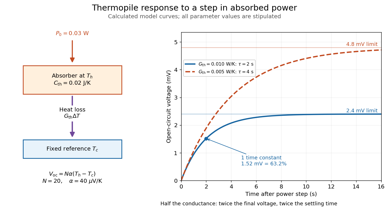
The steady ratio $V_{\infty }/P_0=N\alpha /G_{\mathrm{th}}$ is $0.080\mathrm{V}{\mathrm{W}}^{-1}$ in this constructed model. Halving thermal conductance doubles this ratio but also doubles the time constant if heat capacity stays fixed. Reducing heat capacity alone speeds the response without changing its steady value. Increasing $N$ gives a larger signal only at fixed individual temperature differences: adding legs can also change thermal conductance, heat capacity and electrical resistance. The algebra identifies coupled design choices, rather than predicting a particular manufactured detector.

A finite electrical resistance produces Thermal electrical noise. For nearly uniform absolute temperature $T$ and effective measurement signal bandwidth $B$, its root mean square open-circuit voltage isHere $k_{\mathrm{B}}$ is the Boltzmann constant. Thermal electrical noise in the sensing element is an important contribution, and the signal bandwidth enters its voltage variance.^[ref] If identical pairs have fixed electrical resistance $r$ and fixed $\Delta T$, then $R_{\mathrm{pile}}=Nr$: the signal grows as $N$ while this noise grows as $\sqrt{N}$. The resulting signal-to-noise ratio grows only as $\sqrt{N}$ under those assumptions. Reference temperature drift, environmental electromagnetic radiation, and meter noise remain separate limits; reducing signal bandwidth trades fast information for less integrated electrical noise.

Thermoregulation regulates body temperature. Skin signals can anticipate a change of core body temperature, so a response need not wait for an internal error. ^[ref]

These responses have costs and environmental limits. Shivering consumes metabolic resources; cooling through sweating removes water that must eventually be replaced. High humidity restricts evaporation, so secreted sweat and successful cooling are not interchangeable. Maintaining core body temperature also depends on maintaining circulation: depleted blood volume can compromise skin blood flow and heat transfer. Seeking shade or reducing work changes the disturbance itself, whereas a larger regulatory command merely attempts to counter it. ^[ref]

magnetization retained as magnetic minerals cool through blocking temperatures in an ambient field. Subsequent alteration, reheating and remagnetization can change the record.