Topics (384k) Articles (398k) Users (410) Discussions (242) Comments (383) Files (13k) New article

Metrological traceability is a property of a measurement result: a documented, unbroken sequence of measurement calibrations relates it to a stated reference, and every link contributes to its measurement uncertainty. The reference can be a practical realization of a measurement unit, a measurement procedure or a measurement standard.[ref]
Consider an original mass-measurement chain: a reference measurement standard calibrates a working mass, which is used for instrument calibration of a balance, which weighs an object. Suppose the reference contributes of standard uncertainty, the transfer adds an independent , and the final weighing adds an independent . With unit sensitivity to these additive contributions,The intermediate working mass has of standard uncertainty. That value already includes the reference contribution; adding the same again at the final step would double-count it. Correlated contributions require covariance terms rather than the independent-input calculation.[ref]
Documentation must identify the reference, comparison procedures, dates, applicable conditions and uncertainty contributions. A certificate or instrument label alone does not supply the complete chain for every later result. Metrological traceability also does not ensure that the resulting measurement uncertainty is small enough for the intended use.
A primary measurement standard is a measurement standard established by a primary reference measurement procedure, or an artifact selected by convention. A primary reference measurement procedure obtains its result without calibration against a standard of the same kind of quantity; it may still require measurements of other kinds of quantity.[ref]
For an original ideal pressure realization, independently established force acts on an effective piston area . The measurement model givesIf the inputs have independent standard uncertainties and , first-order propagation of uncertainty givesso . This is an illustrative model, not a complete piston-gauge uncertainty budget: a physical realization must also account for effects such as piston deformation and friction.[ref]
The essential distinction is how the pressure value is established. Merely comparing a gauge with another pressure gauge does not make it a primary measurement standard. Primary status also does not mean zero measurement uncertainty.
An analytical calibration function relates the amount or concentration of an analyte to the expected response of a measurement process under specified conditions. Writing analyte quantity as and observed signal as , a forward model is . IUPAC defines the calibration function through expected gross signal, rather than through an exact noise-free value for each individual reading.[ref]
For an original linear response model, choosein consistent chosen signal/concentration units. A measured signal gives estimate . The inverse conversion is an analytical evaluation function when the forward function is invertible on the calibrated range.[ref] A calibration plot and its inverse computation have different input/output roles.
One way to estimate the relation is to prepare standards with reference concentrations, measure replicate signals, fit a response model and examine calibration residuals. If noise has different variance at different concentrations, an unweighted straight-line fit need not represent the measurement errors adequately. The reference concentrations and preparation procedure also carry measurement uncertainty.
For the linear inverse, first-order error propagation with independent uncertainties in , and givesAt the example estimate, choosing , and gives in concentration units. Treating the fitted coefficients as exact would give only . If the fitted slope and intercept are correlated, their covariance terms must also be included; the displayed formula assumes independence solely for this calculation.
The response need not be linear. An inverse must respect the fitted range and any monotonicity restrictions. Nor does inverting an expected-response curve generally commute with taking an expectation for a nonlinear curve. Measurement calibration supplies a relation and uncertainty model; it does not guarantee that extrapolation, another sample matrix or another instrument state obeys the same function.
Measurement trueness describes how closely the mean of indefinitely many replicate measured values would agree with a reference value. It concerns systematic error, rather than the random spread described by measurement precision. The VIM treats measurement trueness as qualitative: a numerical error or bias estimate is not itself a numerical value of trueness.[ref]
An original measurement model separates the two issues:Here is a fixed offset from the stipulated reference and is random measurement error. Thus , while the standard deviation of individual readings is . For independent random variables following this same model, averaging givesMore readings reduce the random scatter of the mean without removing .
For a stipulated length example, instrument A has and ; instrument B has and . A is more precise, while B's limiting mean agrees better with the reference. With 25 independent readings each, the means have standard deviations and respectively, and their expected offsets remain and zero. These are chosen model parameters, not experimental determinations.
Experimentally, compare repeated readings of a stable measurement standard with its assigned value under specified conditions. A finite observed mean difference estimates an offset; its interpretation includes sampling variation and the reference's measurement uncertainty. Determine an appropriate correction through measurement calibration, apply it in the measurement model, and check it with further reference measurements. Neither a small sample spread nor a single reading equal to the reference establishes measurement trueness.
A measurement model relates the measurand to measured inputs and correction quantities, for example when inferring electrical resistance. Its mathematical form states which physical effects are included in the result.
For small uncertainties, linearization gives . The covariance term shows why shared calibration information matters. A model must also account for effects such as instrumental drift when they materially influence the inference.[ref]
Detector saturation occurs when increasing the input no longer produces the response expected from the detector's lower-input calibration. The limitation may arise in the sensing element, its load circuit, an amplifier or the digitizing stage of the measuring chain. A nearly flat output then represents many different inputs, so the lost amplitude information cannot be recovered by applying the original linear conversion.
A primary physical example is Thorlabs' silicon-photodiode saturation study. It varies reverse bias and load resistance and examines the resulting saturation limit and noise floor. Its stated limitations include testing one FDS100 photodiode with a continuous-wave source; those observations do not establish a universal limit for every detector or pulsed illumination condition.[ref]
Photodiode Saturation and Noise Floor by Thorlabs. Experimental Limitations, p11/12; indexed primary-document text
For an original idealized output-limit model, let incident optical power be andThe linear branch reaches its limit at . Inputs , and all produce in this model. Interpreting that output as therefore reports for each, hiding the differences. The abrupt limit is a teaching model; real response can depart from linearity gradually.
An optical attenuator placed before the detector can provide a check while retaining usable input information. For transmission and original , the detector receives and gives on the linear branch. Correcting the known attenuation recovers . Scaling a clipped stored value after detection cannot perform the same recovery.
To test detector linearity, vary calibrated attenuation or source power while monitoring stability and keeping geometry and wavelength fixed. Compare output ratios, including the background contribution, rather than assuming every output plateau is a constant source. Thorlabs also identifies reverse bias, load and bandwidth as relevant system conditions.[ref]
Photodiodes by Thorlabs. Lab Facts, Photodiode Saturation Limit and Noise Floor, Figures1–3 and accompanying discussion
In the flat part of the ideal response, transducer sensitivity is zero, and the inverse measurement model is no longer unique.Detector linearity describes how consistently a detector's corrected output remains proportional to input over a stated range and under specified conditions. For optical power and output , an affine measurement model is , where is background and is constant. After background subtraction, doubling power should double output. A change in detector responsivity with input level is evidence of departure from that proportional relation.
For an original two-level test, suppose independently established powers are and . A background reading is , while illuminated readings are and . Define the response ratioThe second corrected output is below the doubling expected from the first. Ignoring the background would instead give , confusing offset with nonlinearity. These are stipulated teaching readings, not measured performance of a named detector.
A primary apparatus example is NIST's characterization of a photodiode at . It reports responsivity relative to the low-power value, using a beam splitter to illuminate two photodiodes at about a intensity ratio, with the detector aperture uniformly filled. The report explicitly notes that the observed linearity depends on irradiation geometry.[ref]
Spectroradiometric Detector Measurements: Ultraviolet, Visible, and Near-Infrared Detectors for Spectral Power by Thomas C. Larason and others. 2008edition, §9.1, printed pp85–86, linearity method and Figure9.2
A useful test therefore controls wavelength, beam position and size, bias, temperature, readout gain and source stability while changing input level. Reference-detector nonlinearity or a changing beam ratio can imitate nonlinearity of the test detector. Quantify the uncertainty in the comparison before interpreting a small response-ratio departure.
Detector saturation is a strong limiting case, but detectable nonlinearity can arise before the output becomes flat. A satisfactory response ratio at two levels also does not establish detector linearity over every intermediate level or different operating conditions. Record the tested range and the reference relation with the measurement result.
A ratiometric measurement infers a quantity from a ratio of two measured signals chosen to share an unwanted multiplicative variation. The useful question is which inputs actually share that variation: a reference resistor error or a change in the sensor itself generally survives the cancellation.
In a shared-excitation resistance ratio measurement, a current source passes the same electric current through a sensor of electrical resistance and a reference resistor . Their electric potential differences are and . An ideal normalized analog-to-digital converter reading is thereforeThe current source need not have a perfectly constant output for this cancellation, provided both measurements sample the same electric current, the denominator is nonzero, and the converter stays within its operating ranges. This is a standard arrangement for a resistance thermometer.[ref]
A Basic Guide to RTD Measurements by Joseph Wu. §2.1.3, pp. 10–11, shared-current resistance measurement
For an original ideal example, take , and . Then , and . Increasing by gives and : the ratio remains . If the converter instead uses an independent fixed reference and the calculation assumes the original , the inferred electrical resistance becomes .
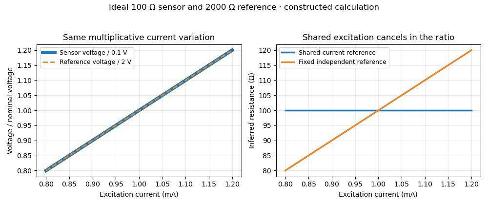
Shared excitation cancels in a resistance ratio; a fixed independent reference retains the excitation error. Original ideal calculation, not measured data.
Details. The reference-resistor error in ratiometric resistance measurement remains even with perfect shared excitation. If the actual reference resistor is but the calculation uses its nominal value, thenThus a reference error makes the nominal estimate of a true sensor about . Reference accuracy and its variation with temperature still matter.[ref]
Nor does the ratio remove sensor self-heating in a ratiometric resistance measurement. Joule heating dissipates , which is in the example. A temperature rise changes the actual electrical resistance of a resistance thermometer; the ratio then measures that changed resistance. Reducing the electric current or comparing several currents can reveal this physical effect.[ref]
The law of propagation of uncertainty makes the role of covariance explicit. For small perturbations of nonzero mean signals, the first-order measurement uncertainty of obeysThe contribution from a shared excitation fluctuation cancels through the covariance term. Treating the two signals as independent random variables would discard that cancellation. Other errors need their own inputs in the complete model.[ref]
For time-varying excitation, ratiometric cancellation with matched signal and reference filters requires matching dynamics as well as shared wiring. With constant resistances and identical linear time-invariant systems of impulse response , the filtered signals are and , so their ratio is still wherever defined. Here denotes convolution. Different filters or different sampling times can leave an excitation-dependent error.[ref]
RTD Ratiometric Measurements and Filtering Using the ADS1148 and ADS1248 Family of Devices by Luis Chioye. First-page abstract and low-pass filter design discussion, matching input and reference filters
A simple proposed bench test first replaces the sensor by a stable calibrated resistor, sweeps the electric current within the instrument limits, and records both electric potential differences and their ratio. That separates electrical cancellation from changing sensor temperature. Repeating with a resistance thermometer in a stable bath then tests Joule heating; changing the reference resistance or one filter tests the predicted failure modes. These are proposed checks of the model, rather than reported experimental results.
MathML Core is a browser-oriented subset of MathML with specified rules for mathematical presentation and layout. The pinned 24 June 2025 document is a Candidate Recommendation Snapshot. It defines a concrete target for implementation, rather than identifying the whole MathML language with one browser's output.[ref]
MathML Core by World Wide Web Consortium. Abstract; Status of This Document; §2.1 elements and attributes
For an original example, encode a typeset fraction surrounded by parentheses as
<math xmlns="http://www.w3.org/1998/Math/MathML"><mrow><mo stretchy="true">(</mo><mfrac><mi>x</mi><mn>2</mn></mfrac><mo stretchy="true">)</mo></mrow></math>. The row has three children: a left mathematical delimiter, the typeset fraction and a right mathematical delimiter. The fraction's children supply numerator and denominator 2.The parentheses are stretchy mathematical operators: their markup requests size-sensitive layout around the fraction. Core specifies operator stretching and row layout; mathematical glyph variants or mathematical glyph assemblies can supply suitable forms.[ref]
MathML Core by World Wide Web Consortium. §§3.2.4.3, 3.3.1.1 and3.3.2: operator layout, stretching and fractions
This illustrates why presenting a formula requires more than placing all its characters on one text baseline.Changing
stretchy="true" to stretchy="false" changes the layout instruction without changing the fraction's two operands. Exact dimensions also depend on the computer font and applicable layout properties. The markup supplies structure and presentation instructions; substituting a numerical value for and evaluating the quotient is a separate operation.An optimization algorithm is a procedure for finding or approximating an optimum of an objective function subject to specified optimization constraints. Its output must be assessed through feasibility, objective quality and a justified stopping rule, rather than only the number of iterations performed.
For , gradient descent with fixed step gives . It converges to the minimizer for , oscillates without decay at when , and diverges for . This elementary example shows why an update formula needs a step-size condition. For a nonconvex objective, a small gradient can certify approximate stationarity without certifying a global minimum.
Combinatorial optimization minimizes or maximizes an objective function over discrete structures such as graph paths, graph matchings, trees or permutations. A weighted minimum spanning tree problem, for example, chooses a tree connecting all vertices and minimizes the sum of its edge weights.
The number of feasible structures can be enormous, but this alone does not prove computational hardness. Minimum spanning trees admit efficient greedy algorithms, whereas the general travelling salesman problem is NP-hard. The useful question is which structural properties allow an algorithm to certify an optimum without explicitly listing every feasible object. Relaxations, dynamic programming and approximation algorithms exploit different kinds of structure.
Stochastic optimization treats optimization involving uncertain quantities or algorithms driven by random observations. A basic model is with , where the decision must be chosen before the relevant realization of is known.
For and finite second moment, the minimizer is . A fresh independent observation supplies , an unbiased estimate of the gradient . A stochastic gradient descent step uses that noisy information rather than evaluating the entire expectation. Averaging or suitable decreasing step sizes can control the accumulated noise; replacing an expectation with one random observation does not make its minimizer the population optimum.
Quasiconvex optimization minimizes a quasiconvex function over a convex set of feasible points. Its defining advantage is that every sublevel set is convex: for each fixed threshold , asking whether a feasible satisfies becomes a convex feasibility problem. The objective function itself need not be a convex function.[ref]
For an original one-dimensional example, minimizeIts derivative is positive, so its sublevel sets on this interval are intervals and the function is a quasiconvex function. Yet , so this nonconstant function is strictly concave rather than convex. For fixed , the denominator is positive, and the threshold condition becomes the linear inequalityAt , no allowed satisfies it; at , the allowed interval does. The true minimum is .
Interval bisection can search thresholds without directly minimizing the original ratio. Maintain an infeasible lower threshold and a feasible upper threshold , with a stored feasible witness for . Test : on feasibility replace and its witness; on infeasibility replace . With exact decisions, after tests the bracket width isStarting with , and witness , the example's first test finds feasible at . Later tests below0.5tighten the lower bound.[ref]
Convex Optimization by Stephen Boyd and Lieven Vandenberghe. Section4.2.5, Algorithm4.1, bisection for quasiconvex optimization
The threshold search is only as reliable as its feasibility problem solver and tolerances. Convexity of the sublevel sets does not supply an inexpensive representation of every such set, and the interval-width guarantee assumes justified feasibility decisions. Returning a feasible witness also matters: an objective bound alone is not an implementable solution.
A feasibility problem asks whether any point satisfies a specified collection of optimization constraints, and seeks such a point when one exists. There need not be a preference among satisfying points. If the feasible set is , the mathematical questions are whether is empty and, if not, how to produce a feasible point. A feasibility problem can be represented as mathematical optimization with a constant zero objective function.[ref]
Convex Optimization by Stephen Boyd and Lieven Vandenberghe. Section4.1.1, printed pp128–129, feasibility problems
For an original linear example, considerThe pair is a directly checkable witness. Replacing the last bound by makes the constraints inconsistent: adding , and gives . This short contradiction certifies infeasibility without enumerating candidate points.
More generally, for a real linear system , a vector satisfyingis an infeasibility certificate: multiplying and adding the assumed inequalities would force . This is the certificate side of Farkas' lemma. A failed numerical search or a timeout is different from such a proof; it need not imply that the feasible set is empty.
The allowed variable set is part of the question. The equation is feasible over the real numbers, with , but infeasible when must be an integer. Thus replacing integer programming constraints by a real relaxation changes the feasibility problem.
Quasiconvex optimization supplies a useful connection: for each threshold , test whether the original constraints and admit a feasible point. Such decisions can bracket the optimal value, while a retained witness gives an actual decision attaining the tested bound.[ref]
Convex Optimization by Stephen Boyd and Lieven Vandenberghe. Section4.2.5, printed pp145–146, Algorithm4.1
Numerical tolerances should be stated: a small constraint residual can support approximate feasibility without proving exact satisfaction.A linear complementarity problem asks for real vectors satisfyingfor a prescribed real matrix and vector . The inequalities hold componentwise. Since every product is nonnegative, the final equality means for every index: each paired component has at least one zero. The linear complementarity problem is a feasibility problem; it need not come with an objective function. Its affine equation does not make the product condition linear.[ref]
Underactuated Robotics by Russ Tedrake. Multi-Body Dynamics, Time-Stepping with hard constraints: definition of the LCP
For an original two-variable example, takeThe pair and satisfies all three conditions. Guessing which member of each pair vanishes reduces the remaining equations to a candidate linear system, but each candidate must still satisfy nonnegativity. Choosing here gives and fails that check. Some data admit no solution: in one dimension, gives for every .
The connection with quadratic programming explains one important tractable case. For a symmetric matrix , considerThe Karush-Kuhn-Tucker conditions set its gradient equal to a nonnegative constraint multiplier and impose complementary slackness, giving precisely the displayed linear complementarity problem. If is a positive-definite matrix, the objective function is strictly convex and grows without bound as , so a unique minimizer exists. This conclusion uses that additional matrix property, not merely the word linear.
There is also a short uniqueness proof. For two complementary pairs,Positive definiteness then forces . This argument gives a directly checkable reason for uniqueness in the stipulated case.
In unilateral contact complementarity, a nonnegative separation pairs with a nonnegative normal contact force: an open gap has zero contact reaction, while a positive reaction requires closed contact. A time-discretized rigid body model can relate its next-step gap affinely to the unknown reaction, producing a linear complementarity problem. The particular discretization and impact law determine that affine relation; the algebraic form alone does not select the physical contact model.[ref]
Pinned article: Introduction to the OurBigBook Project
Welcome to the OurBigBook Project! Our goal is to create the perfect publishing platform for STEM subjects, and get university-level students to write the best free STEM tutorials ever.
Everyone is welcome to create an account and play with the site: ourbigbook.com/go/register. We belive that students themselves can write amazing tutorials, but teachers are welcome too. You can write about anything you want, it doesn't have to be STEM or even educational. Silly test content is very welcome and you won't be penalized in any way. Just keep it legal!
Intro to OurBigBook
. Source. We have two killer features:
- topics: topics group articles by different users with the same title, e.g. here is the topic for the "Fundamental Theorem of Calculus" ourbigbook.com/go/topic/fundamental-theorem-of-calculusArticles of different users are sorted by upvote within each article page. This feature is a bit like:
- a Wikipedia where each user can have their own version of each article
- a Q&A website like Stack Overflow, where multiple people can give their views on a given topic, and the best ones are sorted by upvote. Except you don't need to wait for someone to ask first, and any topic goes, no matter how narrow or broad
This feature makes it possible for readers to find better explanations of any topic created by other writers. And it allows writers to create an explanation in a place that readers might actually find it.
Figure 1. Screenshot of the "Derivative" topic page. View it live at: ourbigbook.com/go/topic/derivativeVideo 2. OurBigBook Web topics demo. Source. - local editing: you can store all your personal knowledge base content locally in a plaintext markup format that can be edited locally and published either:This way you can be sure that even if OurBigBook.com were to go down one day (which we have no plans to do as it is quite cheap to host!), your content will still be perfectly readable as a static site.
- to OurBigBook.com to get awesome multi-user features like topics and likes
- as HTML files to a static website, which you can host yourself for free on many external providers like GitHub Pages, and remain in full control

Figure 2. You can publish local OurBigBook lightweight markup files to either OurBigBook.com or as a static website.
Figure 3. Visual Studio Code extension installation.
Figure 5. . You can also edit articles on the Web editor without installing anything locally. Video 3. Edit locally and publish demo. Source. This shows editing OurBigBook Markup and publishing it using the Visual Studio Code extension. 
- Infinitely deep tables of contents:



All our software is open source and hosted at: github.com/ourbigbook/ourbigbook
Further documentation can be found at: docs.ourbigbook.com
Feel free to reach our to us for any help or suggestions: docs.ourbigbook.com/#contact