Topics (384k) Articles (398k) Users (410) Discussions (242) Comments (383) Files (13k) New article

A measuring chain is one successive signal path through a measuring system, beginning at a sensor and ending at an output element. The VIM illustrates this with both an electro-acoustic chain and a mechanical chain; a measuring chain need not be electronic.[ref]
Consider an original force measurement: a load cell produces an electric potential difference, an amplifier scales that signal, an analog-to-digital converter encodes it, and software converts the code to a force value. This is one measuring chain within the larger measuring system, which also includes its excitation supply, references and mounting arrangements. The load cell acts as a measuring transducer.
In an ideal linear model, let sensor response be , amplifier gain , and converter step per code increment. If the additive output offset is increments, the numerical output isThus implies . These are stipulated teaching values, not measured equipment performance.
The example exposes why measurement calibration must describe the relevant path. Changing amplifier gain changes the relation between output and force even if the load cell is untouched. A saturated stage can also discard information that later conversion cannot restore. Gain uncertainty, offsets, instrumental drift and finite conversion steps contribute at different points; treating the final display's increment as the whole measurement uncertainty overlooks those contributions.
A measuring transducer is a device whose output quantity has a specified relation to its input quantity and is used in measurement. VIM examples include a thermocouple, a strain gauge and a Bourdon tube.[ref] A measuring transducer provides a link in a measuring chain; it need not itself display a finished measurement result.
For an original pressure readout, choose a linear modelwith pressure , output electric potential difference , transducer sensitivity , and offset . An output then corresponds to . An amplifier, analog-to-digital converter and display can follow the transducer, each contributing to the whole measuring system.
The inverse calculation exposes distinct uncertainty contributions. Holding the other inputs fixed, a small output change changes inferred pressure by ; a small offset error changes it by . An output increment corresponds to for the stipulated sensitivity, but does not establish a total measurement uncertainty of that size.
Characterize the relevant range, temperature conditions, response time and possible instrumental drift during measurement calibration. The relation can be nonlinear, in which case local transducer sensitivity is the appropriate derivative rather than one gain valid everywhere. The definition also allows input and output quantities of the same kind; it does not require changing from a mechanical quantity to an electrical one. A sensor denotes the part directly affected by the phenomenon being sensed, whereas a complete measuring chain can contain further measuring transducers.
A Type A evaluation of uncertainty obtains an uncertainty component through statistical analysis of observations. For independent repeated readings with sample standard deviation , the estimated standard uncertainty of their mean is .
Independence and stability matter: serially correlated readings do not generally provide independent pieces of information. Type A and Type B evaluation of uncertainty classify how components are assessed, rather than separating random measurement errors from systematic error.[ref]
A Type B evaluation of uncertainty uses information other than a statistical analysis of repeated observations of the current quantity. Examples include calibration certificates, manufacturer specifications and knowledge of resolution. It describes the evaluation method, not whether an effect is systematic or random.
If a rounding error is reasonably modeled as uniform on , its standard uncertainty is . The distribution assumption is part of the evaluation and should be justified by the available information.[ref]
An expanded uncertainty is , where is the combined standard uncertainty and a stated coverage factor. A result written aims to describe an interval with a specified coverage interpretation.
If a normal approximation is appropriate and the standard uncertainty is well determined, gives approximately 95 percent coverage. This interpretation requires those assumptions; multiplying by two alone does not prove a coverage probability. Report the factor and the basis for its choice.[ref]
A sensitivity coefficient describes how an estimated output of a measurement model changes when one input changes slightly. For , the first-order coefficients, evaluated at the input estimates, areA sensitivity coefficient can have a sign and a unit of measurement: for an output in ohms and an input in volts, its unit is ohms per volt. The GUM also describes estimating sensitivity coefficients experimentally by varying inputs.[ref]
In a measurement uncertainty budget, propagation of uncertainty uses these coefficients to transform input variances and covariances:Here denotes an input standard uncertainty. The derivative's sign disappears from its independent variance term but still matters in a covariance term.[ref]
Evaluation of measurement data — Guide to the expression of uncertainty in measurement by JCGM. Sections5.1–5.2, equations10 and13
For an original electrical resistance example, , and give andIndependent input standard uncertainties of0.1volt and0.02ampere each contribute0.05ohm on the output scale, giving . A larger sensitivity coefficient alone does not identify the dominant uncertainty: the input standard uncertainty and any correlations also matter.
The derivative is a local approximation. If the input spread spans a strongly nonlinear part of the measurement model, first-order propagation of uncertainty can be inadequate even when every derivative has been computed correctly.
A covariance matrix describes second moments, but does not specify a complete probability distribution. A bounded model can realize a prescribed covariance matrix exactly while keeping every possible error finite. This is useful for checking a nonlinear measurement model without accidentally generating physically impossible inputs; it is a constructed model, not evidence that an actual instrument has that distribution.
For two errors with desired standard deviations and correlation coefficient , let be independent random variables with the Rademacher distribution: each takes and with probability . SetBoth expected values vanish. Since and , direct expansion givesThere are at most four distinct states, each obtained from an equally likely sign pair. Also and . At the second sign has no effect, leaving only two distinct states. If either standard deviation is zero, the corresponding error is zero and its correlation coefficient is undefined; the covariance construction still makes sense.
More generally, a finite-support realization of a covariance matrix exists for every real symmetric positive semidefinite matrix . By the spectral theorem, write using its positive eigenvalues and corresponding orthonormal eigenvectors, and put . Let have independent Rademacher distribution coordinates. The random vector then satisfiesThe identity matrix appears because the signs have unit variance and zero pairwise covariance. There are at most distinct states, with component bounds by the Cauchy-Schwarz inequality. When , take . Thus singular covariance matrices are allowed; a nonsingular Cholesky decomposition is not required.
This full sign model also makes robust linear constraints for bounded covariance models exact. To require for every sign state, choose each sign to minimize its contribution. The result is the necessary and sufficient conditionwhere is the L1 norm. This is a small robust optimization calculation. A physical domain must be checked in the chosen units; clipping inadmissible samples afterwards generally changes both the probability distribution and its covariance matrix.
For example, in correlated threshold and amplitude errors in RC timing, take nominal amplitude , threshold , , and . Use and . Every state has , while the minimum amplitude-minus-threshold isAll four states therefore remain within the RC threshold-crossing time domain. Enumerating them supplies an exact check for this particular bounded error model; it does not establish the instrument's actual tail probabilities.
The nonuniqueness of bounded uncertainty laws with a fixed covariance is visible even in two dimensions. LetFor independent fair signs , both and have covariance matrix because is an orthogonal matrix. Yet the first coordinate of is always , whereas that of is with probability and each of with probability . Hence is respectively zero and one half, despite identical expected values and covariance matrices. A nonlinear risk calculation needs more than those moments.
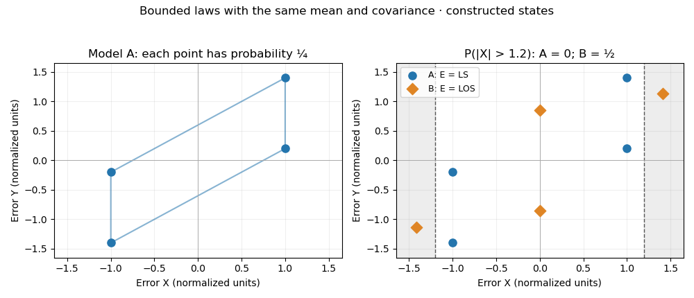
Two bounded four-state error models with identical covariance and different tail probabilities. All points are constructed, not measured data.
Details. A reference material is established as suitable for a specified measurement use because the relevant properties are sufficiently homogeneous and stable. The requirement concerns particular properties and an intended use, rather than every possible attribute of the material.[ref]
International vocabulary of metrology by JCGM. VIM3entry5.13, definition
Reference material homogeneity concerns variation within or between the portions used; reference material stability concerns maintaining the relevant properties over time and under stated conditions.Reference materials can support measurement precision control even without an assigned quantity value. An assigned value is needed when the material serves in measurement calibration or a check of measurement trueness.[ref]
International vocabulary of metrology by JCGM. Entry5.13, note2
A certified reference material adds authoritative documentation specifying property values with associated uncertainties and traceabilities obtained through valid procedures.[ref]A concrete physical example is the archived 2009 certificate for National Institute of Standards and Technology SRM 1922, a mineral oil characterized for refractive index. Its characterization used a precision spectrometer and goniometer arrangement with the minimum deviation method, oil in a hollow optical prism, and water-bath temperature control. Measurements covered several wavelengths and temperatures; multiple portions were examined to assess homogeneity.[ref]
Certificate for Standard Reference Material 1922 by National Institute of Standards and Technology. Certificate issued 24 June 2009, p1, Certified Values and Uncertainties
The certificate's Table 1 reports, at wavelength 589.3 nm and temperature , refractive index 1.46945 with expanded uncertainty and coverage factor 2. This wavelength's value was obtained through a dispersion fit. The listed temperature coefficient is .[ref]
Certificate for Standard Reference Material 1922 by National Institute of Standards and Technology. p1, fitted 589.3nm values and coverage factor; p2, Table1
An original calculation using that linear coefficient predictsThe predicted change, in magnitude, is larger than the quoted expanded uncertainty at the reference conditions. Temperature therefore belongs with the assigned optical value; it is not an incidental label. This calculation illustrates the certificate's model, rather than supplying a new certified value or uncertainty.
Record the material identity, certificate version, property, wavelength, temperature and handling history with a measurement result. The archived certificate supplies a documented example of those links, rather than a claim about a currently available product or the validity of a particular bottle today.
A measured quantity value is a value used to represent a measurement result. It may be obtained from one observation or calculated from replicate observations, for example as an arithmetic mean. The VIM distinguishes this value from a raw measurement indication and from the fuller result with its measurement uncertainty.[ref]
International vocabulary of metrology by JCGM. VIM3entry2.10, definition, note1 and annotation9December2016; entry2.9, note2
For an original electrical resistance example, suppose three instrument indications are , and . A measurement calibration gives additive indication offset , so the corrected values are , and . Their arithmetic mean is the representative measured quantity valueThis value is a numerical estimate of the specified measurand, such as the resistor's resistance at a stated temperature. It is not established as an exact true value merely by correcting the indications.
The three values have sample standard deviation . If repeat deviations are independent, their contribution to the mean's standard uncertainty is . Suppose the common correction has independent standard uncertainty . First-order propagation of uncertainty givesRepeating the readings reduces the first term under these assumptions; it does not repeatedly remeasure and average away the same common correction. These are illustrative uncertainty inputs, not observed equipment data.
Reporting the measured quantity value therefore requires its unit and measurand definition. Reporting the complete measurement result also identifies the associated measurement uncertainty, its convention and relevant conditions. A change from ohms to milliohms changes the numerical expression, while leaving the represented physical value unchanged.
A measurement indication is the value supplied by a measurement instrument or measuring system. It may appear as a pointer position, displayed number, printed output or transmitted code. The indication and the corresponding measurand value need not be values of the same kind of quantity.[ref]
For an original mechanical readout, suppose the indicated pointer position is a length , related to input pressure byThe measurement indication then corresponds to under this measurement model. The position is observable; the pressure value is inferred using the response relation. A printed pressure scale could carry out part of that conversion physically without changing the underlying distinction.
If the pointer position is uncertain by , that contribution corresponds to in this stipulated linear model. Uncertainty in the zero , transducer sensitivity , temperature response and instrumental drift can add further contributions. Closely spaced scale markings therefore do not establish the total measurement uncertainty.
Record the original indication and instrument settings when applying corrections. A corrected measured quantity value can change after improved measurement calibration even though the recorded indication remains the same. For example, revising the assumed zero from to changes the inferred pressure from to . The complete measurement result accompanies the inferred value with its uncertainty and relevant conditions; the raw measurement indication alone cannot supply that information.
Design resolution is the theoretical smallest commanded movement implied by a positioning mechanism's drive components. For a screw drive, it can be calculated from screw pitch, reduction gearing and motor or encoder increments. It is not automatically the minimum incremental motion that the final load executes repeatedly.[ref]
For an original ideal drive, let a lead screw advance per revolution, with 50 motor revolutions per screw revolution and 2000 resolved counts per motor revolution. One count corresponds toDoubling the count resolution to 4000 per motor revolution gives theoretical without changing the screw. That calculation does not halve friction or remove backlash. A controller may display both increments even if the load moves only after several such commands have accumulated.
Keep the location and counting convention of the feedback sensor explicit. Counts at a motor shaft, counts at a screw and directly measured load position are different observations. A gearbox can introduce compliance between them. Pair the design calculation with an independent motion test to establish operational performance. A smaller theoretical increment also does not by itself establish absolute positioning accuracy or a smaller measurement uncertainty.
Minimum incremental motion is the smallest displacement increment that a positioning system can execute repeatedly for the specified input and test conditions. It is an operational motion property, whereas design resolution is derived from the drive geometry and electronic increments. Friction, stiction, elasticity and backlash can make them differ.[ref]
Precision Motion and Positioning: Difference between Micropositioning and Nanopositioning by Physik Instrumente. Glossary, Design Resolution and Minimum Incremental Motion
For an original illustrative test, independently measure the displacement produced by repeated commands from equivalent starting conditions. A nominal 10 nm command gives moves . Their mean is 10 nm, but that mean does not show repeatable 10 nm increments. A nominal 40 nm command instead gives .
Define an example acceptance rule before testing: every measured move must lie within 5 nm of the command, and the readout must have sufficiently smaller uncertainty, stipulated here as 1 nm standard uncertainty. The 10 nm trials fail this rule; the 40 nm trials pass. Among these two candidate increments, 40 nm is the smallest accepted one. It is not a proof of the globally smallest achievable increment because intermediate candidates and other conditions were not tested.
Report the command convention, load, motion direction, starting procedure, displacement sensor, measurement uncertainty and acceptance rule. A rotary encoder on the motor does not automatically measure the final load motion. Independent readout, for example with an interferometer, tests the assembled stage rather than only the commanded count. Positioning repeatability at a target and the ability to make a small move are related but distinct properties.
Input-referred noise expresses observed or modeled output noise as an equivalent disturbance at a system's input. For a locally linear response with constant nonzero gain over the relevant measurement band, an output-noise root mean square corresponds toThis is a way to compare noise with the input signal; it does not locate every physical noise source at the input. Walt Kester's ADC tutorial explicitly models converter noise as an equivalent series input source and describes its measurement through repeated codes under a fixed input.[ref]
For an original amplifier with voltage gain , output noise rms is equivalent to rms at the input. Changing gain can change this quotient without removing the device's own physical noise. State the measurement bandwidth and processing, since a longer averaging interval or different filter changes the observed rms value.
An original two-stage example shows why the position of noise matters. Let gains be and independent input-equivalent noise contributions be for the respective stages. The output-noise variance isso referring it to the original input givesWith , and , this is . Increasing to reduces the equivalent total to about , approaching the first-stage contribution. The independent-noise assumption matters; correlated contributions require covariance terms.
A quiet output code does not by itself establish a small total error, and rms noise is not the same criterion as input-referred resolution. Kester distinguishes noise-based resolution from dynamic converter measures and notes the conditions needed for averaging to help.[ref] Retain offsets, gain uncertainty and instrumental drift separately in the measurement model.
Measurement repeatability is measurement precision under a declared set of repeatability conditions. The VIM's repeatability condition of measurement includes the same procedure, operators, measuring system, operating conditions and location, with repeated measurements over a short time.[ref] The complete measurement cycle must be specified before its repeatability can be assessed.
For an original length-comparator study, one operator measures the same reference block using the same differential length comparator over a short session. Three readings without disturbing the setup happen to be . Their sample spread is zero. In a separate series, the operator removes and reseats the block for every trial, obtaining . That series givesThe two procedures repeat different parts of the experiment. The first data cannot establish the repeatability of the full remove-and-reseat procedure, nor does its zero observed spread prove an absence of readout noise or finite measurement resolution.
A repeatability experiment keeps the declared conditions stable and records each completed trial, including placement and settling when those belong to the procedure. Positioning repeatability applies this reasoning to repeated returns of a moving stage. Repeating a study over longer periods with selected changes can instead assess intermediate measurement precision; studies changing locations, operators and measuring systems concern measurement reproducibility.[ref]
International vocabulary of metrology by JCGM. VIM3entries2.22–2.25, changed and unchanged conditions
Report those changes rather than describing every repeated experiment as the same repeatability test.Intermediate measurement precision is measurement precision under declared intermediate precision conditions of measurement. The measurement procedure and location remain the same, measurements extend over a longer period, and specified changes can include operators, measuring systems or measurement calibration. It lies between a tightly restricted measurement repeatability study and a comparison across locations for measurement reproducibility.[ref]
International vocabulary of metrology by JCGM. VIM3 entries 2.22–2.23, definitions and entry 2.22 notes 1–2
For a concrete study, one laboratory could measure the same stable reference block each working day with a differential length comparator, taking four complete placements per day. Keep the procedure fixed, record temperature and operator, and retain the day labels. The labels let the study distinguish variation between days from rapid reading-to-reading variation.
An original measurement model makes that distinction explicit:Here is a shared daily offset, while varies between placements. Assume zero-mean independent random variables, independent also between days. A single measurement then has standard deviation . For stipulated and , this is , even though within-day scatter reflects only .
For four readings from one day, the daily arithmetic mean hasAveraging four such means from independent days reduces that modelled standard deviation to . Four same-day readings do not average away their shared daily offset. The numbers illustrate the model, not measured comparator performance. A real study must estimate its components from enough days and investigate trends: deterministic instrumental drift is not automatically an independent daily offset.
Measurement reproducibility is measurement precision under specified reproducibility conditions of measurement. These include changed locations, operators and measuring systems; the measurement procedures may also differ. The comparison must state what changed and what remained common.[ref]
International vocabulary of metrology by JCGM. VIM3 entries 2.24–2.25, definitions and entry 2.24 notes 1–2
This is a metrological use of reproducibility, concerned with agreement of measured values under declared conditions.An original comparison sends a stable reference block to three laboratories. Each laboratory uses its own differential length comparator and operator, measures the same specified measurand, and reports three length errors relative to the common reference, in micrometres:Each laboratory has sample standard deviation , yet their arithmetic means differ by as much as . Relative to the grand mean , the total squared deviation separates into within-laboratory and between-laboratory terms:Consequently the nine chosen values have pooled sample standard deviation . This is a descriptive statistic for these observations, not a universal estimator prescribed by the definition of measurement reproducibility. Reporting only the three within-laboratory spreads would conceal the disagreement.
The physical comparison must also monitor transport damage, reference stability and temperature corrections. A changing reference block could imitate a laboratory difference. Measurement reproducibility alone does not establish measurement trueness: all laboratories could share the same erroneous reference value or correction. The changed apparatus and conditions belong alongside the reported statistic.
A null measurement method adjusts a reference or a system setting until a difference signal is brought to zero. A null detector tests the residual mismatch; the final measured quantity value follows from the reference and the balance condition. The VIM lists null measurement among measurement methods.[ref]
A Wheatstone bridge provides a concrete electrical apparatus. The PHYWE manual connects a source across two resistor dividers and a current detector between their middle junctions; balance occurs when those junction potentials agree and detector current vanishes.[ref] A sliding-wire implementation adjusts the divider ratio continuously.
For an original notation, let the left branch contain upper resistance and lower , while the right contains upper unknown and lower reference . With source electric potential difference and negligible loading at balance, the middle-junction potentials above the lower supply terminal areSetting yieldsFor , and , the balance identifies independently of the nonzero source magnitude in this ideal model.
Zero on a display has finite meaning. With , the derivative of residual with respect to at this balance is . A residual magnitude below therefore corresponds locally to about of unresolved mismatch. A detector zero offset can also shift the apparent balance. The null measurement method reduces reliance on calibrated detector gain at exact balance, but reference uncertainties, lead effects, detector sensitivity and instrumental drift remain relevant to the complete measurement result.
A substitution measurement method compares an unknown with a reference by placing them successively in the same relevant position of a measuring system. The comparison seeks a match or measures a difference while retaining as much of the system response as possible. The VIM lists substitution among measurement methods; the detailed sequence belongs to the measurement procedure.[ref]
For a physical application, NIST's double substitution weighing procedure compares a standard and an unknown of the same nominal mass twice, using a weighing instrument as a comparator. It also determines response with a known sensitivity mass and includes measurement-assurance checks.[ref]
Weighing by Double Substitution by National Institute of Standards and Technology. SOP4–2019, p1, Purpose; pp6–8, weighing sequences and observations
The measurement standard supplies the reference value; the comparator need not establish the whole mass independently from its own zero.An original simplified drift model shows why sequence matters. Let a comparator indication at equally spaced time index bewith fixed response coefficient , additive offset and linear instrumental drift . Observe standard S at , unknown X at , and S again at . The mean X indication and mean S indication have the same mean time , givingBoth the constant offset and the stipulated linear drift cancel. For , , and , an unknown gives indications . Their paired means differ by two, recovering .
This teaching sequence isolates one cancellation mechanism; it is not the full NIST procedure. Nonlinear drift, unequal timing, changing response or different positioning can defeat it. NIST's procedure separately addresses buoyancy and uncertainty contributions.[ref]
Weighing by Double Substitution by National Institute of Standards and Technology. SOP4–2019, §3, calculations; uncertainty section, air-buoyancy and density contributions
A close match does not remove the reference's measurement uncertainty or establish that the substitution left every relevant condition unchanged.Polarity reversal measurement separates a signal that changes sign on reversal from an additive contribution that does not. If readings in two polarities obeythen the half-difference estimates the signal, , while the half-sum estimates the unchanged offset, . The procedure depends on reversing the intended signal while preserving the relevant offset.
A primary electrical application is cancellation of thermoelectric offset in low-level measurements. The Keithley handbook describes reversing sources when comparing small electric potential differences, and reversing test current for low-electrical resistance measurements. A thermal offset can arise at dissimilar-metal junctions and remain approximately unchanged during a sufficiently short cycle.[ref]
For an original resistance example, a bipolar current source applies and to a resistor while a voltmeter measuresLet and readings be and . Their half-difference is , giving ; their half-sum reveals a offset. Using only the positive reading would instead give .
An offset changing from to leaves resistance error . A change in this example therefore leaves error. Allow electrical settling after reversal while keeping the cycle short relative to material temperature changes. The handbook explicitly notes this time-scale requirement.[ref]
Low Level Measurements Handbook, Seventh Edition by Keithley Instruments. §3.3.2, current-reversal method, thermal-time-constant limitation
Reversal does not automatically remove lead resistance, current-magnitude errors, self-heating or every offset in the circuit. Record the actual reversal operation and timing with the measurement procedure.Gravimetric dilution determines a dilution from measured masses. A measured amount of a stock solution is combined with material containing none of the quantity being diluted. For a closed transfer and a homogeneous mixture, the conserved amount divided by the final mass determines the new mass-based concentration.
Let be the stock's net mass, the added net mass, and . Define the stock fraction and the gravimetric dilution factor byIf the stock has solute mass fraction , thenFor stipulated , and , the final mass is , , and : 2% by mass. The solute mass is before and after dilution. The net masses exclude their containers. This mass basis does not require an assumption that liquid volumes add.
The uncertainty of a gravimetric dilution depends on which readings share errors. For independently evaluated inputs , first-order propagation of uncertainty givesHere denotes standard uncertainty. The sensitivity factors follow from the partial derivatives and . With a chosen independent at the example's nominal masses, the relative mass-ratio contribution is approximately 0.0453%. Adding an independent 0.5% relative stock-value contribution in quadrature gives approximately 0.502%. These are illustrative inputs, rather than a balance specification.[ref]
Guidelines for Evaluating and Expressing the Uncertainty of NIST Measurement Results by Barry N. Taylor and Chris E. Kuyatt. Section5 and AppendixA: first-order combination, sensitivity coefficients and covariance terms
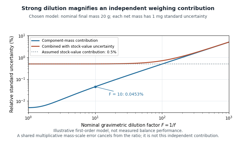
Original first-order uncertainty model for gravimetric dilution: at a fixed nominal final mass, strong dilution increases the relative contribution of independently uncertain component masses
. Details. If input errors have covariance, their cross terms must be retained. A useful exact check isA common multiplicative mass-scale factor therefore cancels from . Counting it as two independent contributions would lose that correlation. Container subtraction, transfer losses and changes in composition require their own assessment; this cancellation establishes only the common-scale property.
For massic activity, the same conservation argument applies after expressing all activities at a common reference time. A 2000 NIST study compared massic activity ratios inferred from gravimetric dilution with independent liquid scintillation counting. Their agreement within reported uncertainties provided an experimental check on transferring standards through mass ratios.[ref]
Massic Activity Ratios of the NBS/NIST Tritiated-Water Standards Issued Between 1954 and 1999 by L. L. Lucas. Abstract and Section3: measured ratios compared with gravimetric dilution factors
Pinned article: Introduction to the OurBigBook Project
Welcome to the OurBigBook Project! Our goal is to create the perfect publishing platform for STEM subjects, and get university-level students to write the best free STEM tutorials ever.
Everyone is welcome to create an account and play with the site: ourbigbook.com/go/register. We belive that students themselves can write amazing tutorials, but teachers are welcome too. You can write about anything you want, it doesn't have to be STEM or even educational. Silly test content is very welcome and you won't be penalized in any way. Just keep it legal!
Intro to OurBigBook
. Source. We have two killer features:
- topics: topics group articles by different users with the same title, e.g. here is the topic for the "Fundamental Theorem of Calculus" ourbigbook.com/go/topic/fundamental-theorem-of-calculusArticles of different users are sorted by upvote within each article page. This feature is a bit like:
- a Wikipedia where each user can have their own version of each article
- a Q&A website like Stack Overflow, where multiple people can give their views on a given topic, and the best ones are sorted by upvote. Except you don't need to wait for someone to ask first, and any topic goes, no matter how narrow or broad
This feature makes it possible for readers to find better explanations of any topic created by other writers. And it allows writers to create an explanation in a place that readers might actually find it.
Figure 1. Screenshot of the "Derivative" topic page. View it live at: ourbigbook.com/go/topic/derivativeVideo 2. OurBigBook Web topics demo. Source. - local editing: you can store all your personal knowledge base content locally in a plaintext markup format that can be edited locally and published either:This way you can be sure that even if OurBigBook.com were to go down one day (which we have no plans to do as it is quite cheap to host!), your content will still be perfectly readable as a static site.
- to OurBigBook.com to get awesome multi-user features like topics and likes
- as HTML files to a static website, which you can host yourself for free on many external providers like GitHub Pages, and remain in full control

Figure 2. You can publish local OurBigBook lightweight markup files to either OurBigBook.com or as a static website.
Figure 3. Visual Studio Code extension installation.
Figure 5. . You can also edit articles on the Web editor without installing anything locally. Video 3. Edit locally and publish demo. Source. This shows editing OurBigBook Markup and publishing it using the Visual Studio Code extension. 
- Infinitely deep tables of contents:




All our software is open source and hosted at: github.com/ourbigbook/ourbigbook
Further documentation can be found at: docs.ourbigbook.com
Feel free to reach our to us for any help or suggestions: docs.ourbigbook.com/#contact