
Heat capacity of a classical magnetic dipole 2026-10-18
A freely orientable classical magnetic dipole moment of fixed magnitude in a uniform magnetic field has angular canonical partition function , where . Its internal energy is , and its fixed-field heat capacity is . At low temperature, two locally Cartesian tangent coordinates on the orientation sphere each contribute by the equipartition theorem, giving . A discrete quantum spin in a nonzero magnetic field instead has a spectral gap and its heat capacity vanishes exponentially at sufficiently low temperature.
One-dimensional entropic chain force-extension relation Created 2026-10-18 Updated 2026-11-05
For independent links pointing left or right with length , fixed signed extension gives and . The multiplicity is when these counts are nonnegative integers. Leading Stirling's approximation gives as the externally applied tension conjugate to . Its small-extension limit is . At fixed tension, the exact one-link partition function is and the mean extension is , confirming the same inverse relation without using Stirling at the full-extension endpoint.
Statistical segment length Created 2026-10-18 Updated 2026-11-05
An effective step length describing a specified chain-count convention: an ideal polymer with counted units has mean-squared end-to-end distance of a polymer chain . If counts freely jointed coarse-grained units, is their Kuhn length. If counts chemical repeat units, the effective incorporates local conformational correlations and is not automatically a physical monomer diameter. A repeat-unit volume is independent information; setting is a scaling approximation.
IceCube-170922A multimessenger association 2026-10-18
The 2018 collaboration paper associated the 22 September 2017 neutrino alert with the flaring blazar TXS 0506+056 through directional and multiwavelength observations. Its approximately evidence included trial corrections and assumed relationships between neutrino and gamma ray emission. A single association did not establish a production mechanism or explain the entire diffuse neutrino flux.[ref]
Multi-messenger observations of a flaring blazar coincident with high-energy neutrino IceCube-170922A by IceCube Collaboration and others. The neutrino alert; Neutrino-blazar coincidence analysis; Discussion, PDF pp. 2–3, 11–13, 62–66
Neutrino directional-coincidence model 2026-10-18
How much does a small directional uncertainty help? Consider an original idealized model: a source direction fixed in advance, uniform background directions over the full sphere, and circular acceptance radius . The accepted solid angle and single-event background probability areThe derivation integrates the area element on a unit sphere. For small in radians, : halving the radius quarters the accidental acceptance, to leading order. At acceptance vanishes; at it covers the full sphere. The solid angle has units of steradians; is dimensionless.
For , take a deliberately crude point spread function: stipulate that every signal direction lies uniformly inside that cap. The signal and background probability density functions per steradian are inside the cap and zero outside, and everywhere. Both integrate to one. For an event inside the cap their likelihood ratio isThis ratio compares two specified directional models; it is not the probability that the event came from the source. Such a conditional probability would additionally require prior source odds and the other selection information. For fixed source fraction among selected events, a normalized mixture distribution has density . For independent events the likelihood is the product of those densities; its ratio to background alone isOutside-cap events contribute factors rather than being silently discarded. At , ; for a full-sky cap, and every gives . A directional model that cannot distinguish source from background carries no directional evidence.
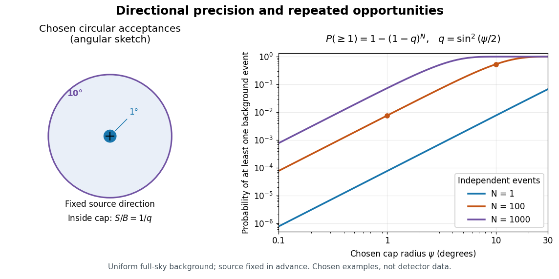
Chosen angular acceptance, directional likelihood and repeated background opportunities
. Original exact spherical-cap calculation and uniform-cap signal model. Radii and event counts are chosen illustrations, not IceCube angular resolutions or discovery data. The fixed source direction and independent uniform background assumptions are essential. Details.
As an original numerical example, radii and give and , respectively: nearly a hundredfold difference. For a fixed number of independent background events, the binomial distribution givesWith chosen , those radii give approximately and . A small single-event acceptance can become a common coincidence after many opportunities. This probability concerns a fixed cap, rather than a scan for the most favorable cap anywhere. For independent searches with common local tail probability , the corresponding global tail probability is ; overlapping sky searches generally violate that independence. Actual source tests must include directional response, nonuniform exposure, energy information and the look-elsewhere effect in their null calibration.
In live days during 2010–2012, events exceeded the expected atmospheric events. Energy, direction and topology supported an extraterrestrial component. Combined searches gave with additional benchmark charm background; uncertain charm production affected significance. No source clustering was established.[ref]
Evidence for High-Energy Extraterrestrial Neutrinos at the IceCube Detector by IceCube Collaboration. Results; Discussion; Search for Neutrino Sources
A diffuse excess and an identified source answer different questions. The first compares populations against a background hypothesis; the second needs an association in direction, perhaps also in time.
IceCube starting-event veto 2026-10-18
The 2013 selection rejected early boundary light. Tagged muons checked leakage; air shower companion muons also vetoed downward atmospheric neutrinos.[ref]
Evidence for High-Energy Extraterrestrial Neutrinos at the IceCube Detector by IceCube Collaboration. Event Selection; Atmospheric Muon Background
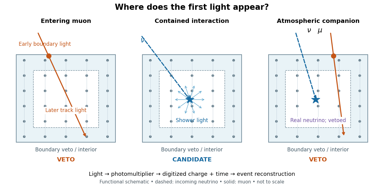
Entering tracks, contained interactions and an accompanying-muon veto
. Original schematic, not to scale or measured data. Dots: optical modules. Dashed arrows: unseen neutrinos; solid arrows: muons. Details.
A simple original conditional probability model explains why a veto changes the selected mixture. Let mean that an atmospheric neutrino interaction would pass all other cuts, that an accompanying muon reaches the veto, and that the veto fires. Set and , and neglect unrelated veto hits. The law of total probability givesFor chosen and , the passing fraction is . Neither this value nor either input is an IceCube measurement. With equal incident candidate populations, this mechanism alone reduces the atmospheric contribution relative to a hypothetical population having . It does not make every surviving event astronomical: or gives no suppression, while removes the entire chosen atmospheric population. If unrelated light vetoes a surviving event independently with probability , its passing fraction becomes ; independence is an additional assumption.
In the 2013 calibration study, six horizontal light-emitting diodes per module on string 63 flashed sequentially; other strings recorded charges and photon arrival times. A global fit inferred depth-dependent scattering of light and absorption coefficients. Dust-logger measurements checked layer structure; independent muon events tested simulated time patterns. Photomultiplier response and refrozen ice near modules remained limitations. Thus a late hit need not imply a late interaction: scattering of light changes the path.[ref]
Measurement of South Pole ice transparency with the IceCube LED calibration system by IceCube Collaboration. Sections 3, 8–11; Figs. 14, 20–23: flashing, cross-checks and limitations
An original limiting calculation isolates this issue. Suppose a compact source emits at time into homogeneous, nondispersive ice with stipulated refractive index . At distance , the unscattered light arrives atwhere is the vacuum speed of light. For chosen , the delay is . A scattered path longer adds even with perfect clocks. These chosen values are not calibration measurements. Real ice requires wavelength-dependent propagation, module response and a spatially varying light-transport model; replacing that response by one arrival time discards information.
Digital optical module 2026-10-18
A glass-enclosed photomultiplier with local digitization: pulse times and charges enter event reconstruction. Reciprocal electrical pulses synchronize module clocks to the surface time base.[ref]
The IceCube Neutrino Observatory: Instrumentation and Online Systems by IceCube Collaboration. Sections 2.1, 3.3: module and reciprocal timing
Weak charged current interactions of muon neutrinos usually give extended muon tracks. Compact particle showers occur in other channels, including weak neutral current interactions of every neutrino flavor. Tracks generally constrain direction better; escaping particles complicate energy inference.[ref]
The IceCube Neutrino Observatory: Instrumentation and Online Systems by IceCube Collaboration. Section 1.1.1: tracks and showers
Work by Ian R. Lanza 2026-10-18
For an infinitely long circular cylinder of uniform mass density , the gravitational Poisson equation and the divergence theorem give internally. The hydrostatic equilibrium equation and boundary value then give the title formula. This model neglects rotation, surface tension and end effects.
Isothermal sphere 2026-10-18
An isothermal sphere is a spherically symmetric self-gravitating gas equilibrium with equation of state and constant . The hydrostatic equilibrium equations and yield the title equation. Its regular finite-central-density solution is distinct from the singular isothermal sphere. A finite outer radius requires confinement because the regular density does not vanish at finite radius.
Luis Walter Alvarez's program extended the Glaser bubble-chamber experiment into large hydrogen bubble chambers and systematic analysis. His lecture credits John G. Wood, an accelerator technician, with early hydrogen tracks, and emphasizes technicians' responsibility for chamber development.[ref]
Recent Developments in Particle Physics by Luis Walter Alvarez. Recent Developments in Particle Physics, lecture 11 December 1968; institutional report UCRL-18696, printed pp. 12–16, Fig. 2
Alvarez's 1956 report describes a ten-inch hydrogen bubble chamber in a steady magnetic field, exposed to a negative-pion beam for proton scattering. Liquid hydrogen was the target. Horizontal windows admitted illumination and stereo viewing; a shielded light source let bubble-scattered light reach the lenses. A temperature gradient initially restricted sensitivity near the top. Tilting and fast recompression improved uniformity.[ref]
Liquid Hydrogen Bubble Chambers by Luis Walter Alvarez. Liquid Hydrogen Bubble Chambers, UCRL-3367, 4 April 1956, PDF pp. 5–7: ten-inch chamber, optics, recompression and scattering exposure
The same report compares tracks without a magnetic field against straightness expectations, testing spurious curvature. Multiple Coulomb scattering remained a limitation. This separates an instrumental check from the physical momentum inferred with the field on.[ref]
Liquid Hydrogen Bubble Chambers by Luis Walter Alvarez. UCRL-3367, PDF p. 7, paragraph beginning “The no field tracks”
The scientific opportunity is to turn a visible geometry into a test of an invisible intermediate state. The bubble-chamber pressure cycle prepares the sensitive target; bubble-chamber track readout supplies geometric measurements. Neither step alone identifies a particle resonance.
Refraction from secondary wavelets Created 2026-10-18 Updated 2026-11-05
Let a plane incident wavefront first meet a flat interface at , and let another point on that front reach on the interface after . Its path has length . The secondary wavelet from has radius in the second medium; the new wavefront through is tangent to it at . Right triangles with common hypotenuse give and , where both ray angles are measured from the interface normal. Consequently , which is Snell's law. The construction uses phase velocities in homogeneous isotropic media.
Relative humidity Created 2026-10-18 Updated 2026-10-31
Relative humidity is the ratio of the partial pressure of water vapor to its saturation vapor pressure at the same temperature, usually expressed as a percentage.
Work by Hui Guo Created 2026-10-18 Updated 2026-10-31
Spin isomers of hydrogen Created 2026-10-18 Updated 2026-10-20
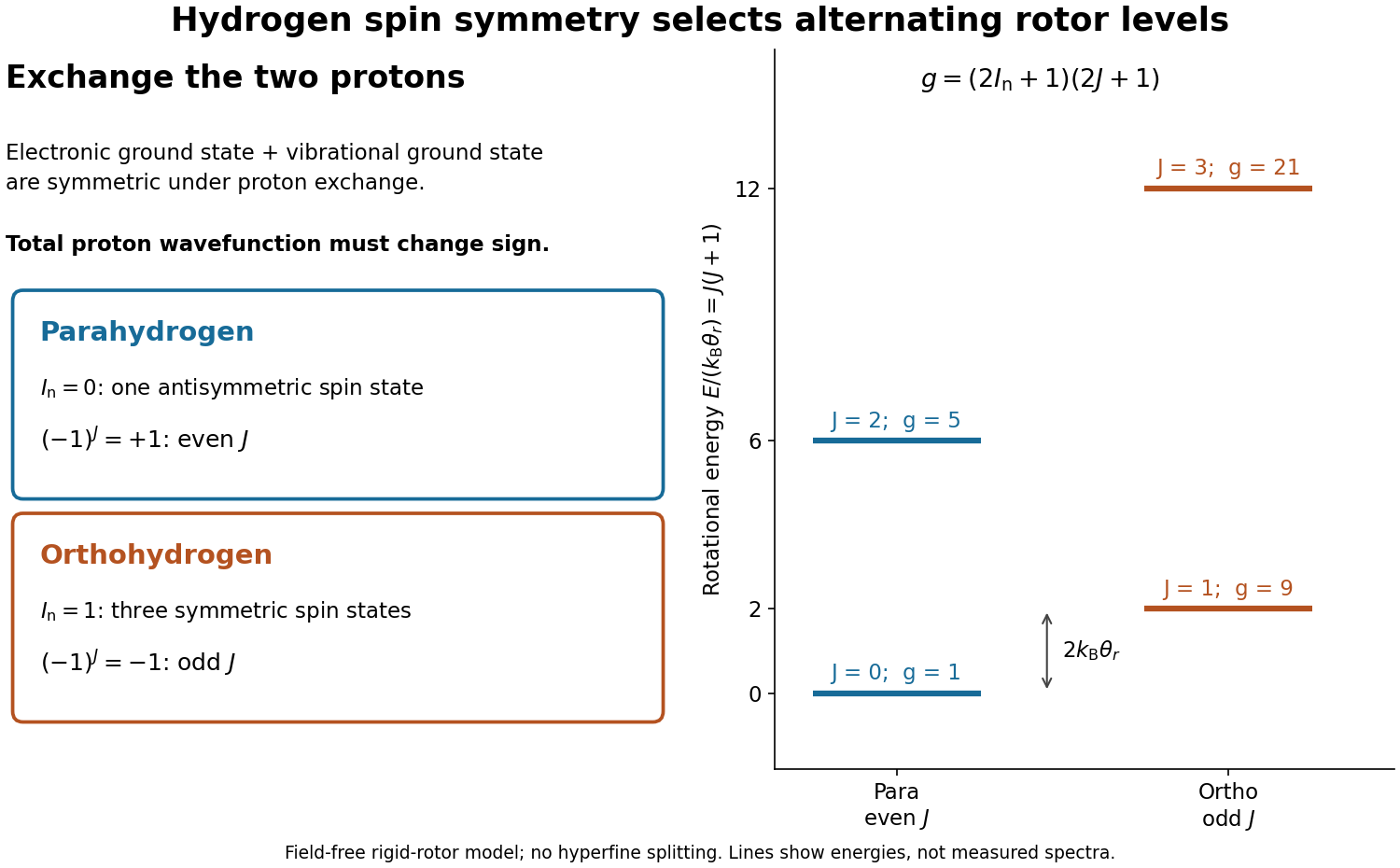
Spin isomers of hydrogen are two forms of molecular hydrogen, , distinguished by the combined nuclear spin of their two protons. They have the same chemical formula and electronic ground state, but different allowed molecular rotation states. Parahydrogen has total nuclear spin zero and even rotational quantum number ; orthohydrogen has total nuclear spin one and odd . The difference makes heat capacity a probe of fermionic exchange symmetry, and makes cooling history matter for a tank of molecular hydrogen.
Assume the electronic ground state and the vibrational ground state of a free molecule. The electronic factor is symmetric under exchanging the two protons, and the vibrational factor depends only on their separation, so it is also symmetric. These assumptions concern the exchange of protons; the electronic wavefunction separately obeys fermionic exchange symmetry under exchange of electrons. Neglect electronic excitation, vibrational excitation, external fields, and small interactions involving nuclear spin when calculating rotational energy eigenvalues.
The two protons are identical particles with spin . Their complete wavefunction must change sign under their particle exchange operator. Interchanging the two ends reverses the internuclear direction , and the spherical harmonic rotational factor satisfiesThe antisymmetric spin-one-half singlet state therefore requires symmetric, even- rotation; the symmetric spin-one-half triplet state requires antisymmetric, odd- rotation. This is exchange symmetry of two identical spin-one-half fermions applied inside a diatomic molecule, not an extra rotational force. A linear rigid rotor may omit spin-dependent splittings while still requiring this restriction on its allowed quantum states.

Off-axis holography 2026-10-18
Off-axis holography tilts the holographic reference wave relative to the holographic object wave. Its interference fringes acquire a carrier spatial frequency; the two cross terms occupy different spatial frequency regions when the carrier is sufficiently large compared with the object's signal bandwidth. This permits filtering a single image term.
Gabor's lecture credits Emmett Leith and Juris Upatnieks with the later skew-reference method using helium–neon laser illumination, separating reconstructed images angularly.[ref]
Holography, 1948-1971 by Dennis Gabor. Gabor, Nobel lecture, Fig. 8 and surrounding account of the 1962–1963 laser work
For an original periodic calculation, let run over a unit-length interval and chooseAll spatial frequencies here are cycles per unit length; the data are a chosen field at the recording plane, not measurements or a physical object profile. Direct expansion givesConsequently its Fourier series coefficients are at zero, at , at and at . The component lies at ; the component lies at ; the background lies at . Filtering the negative-frequency cross term and multiplying by recovers , including its relative wave phase.
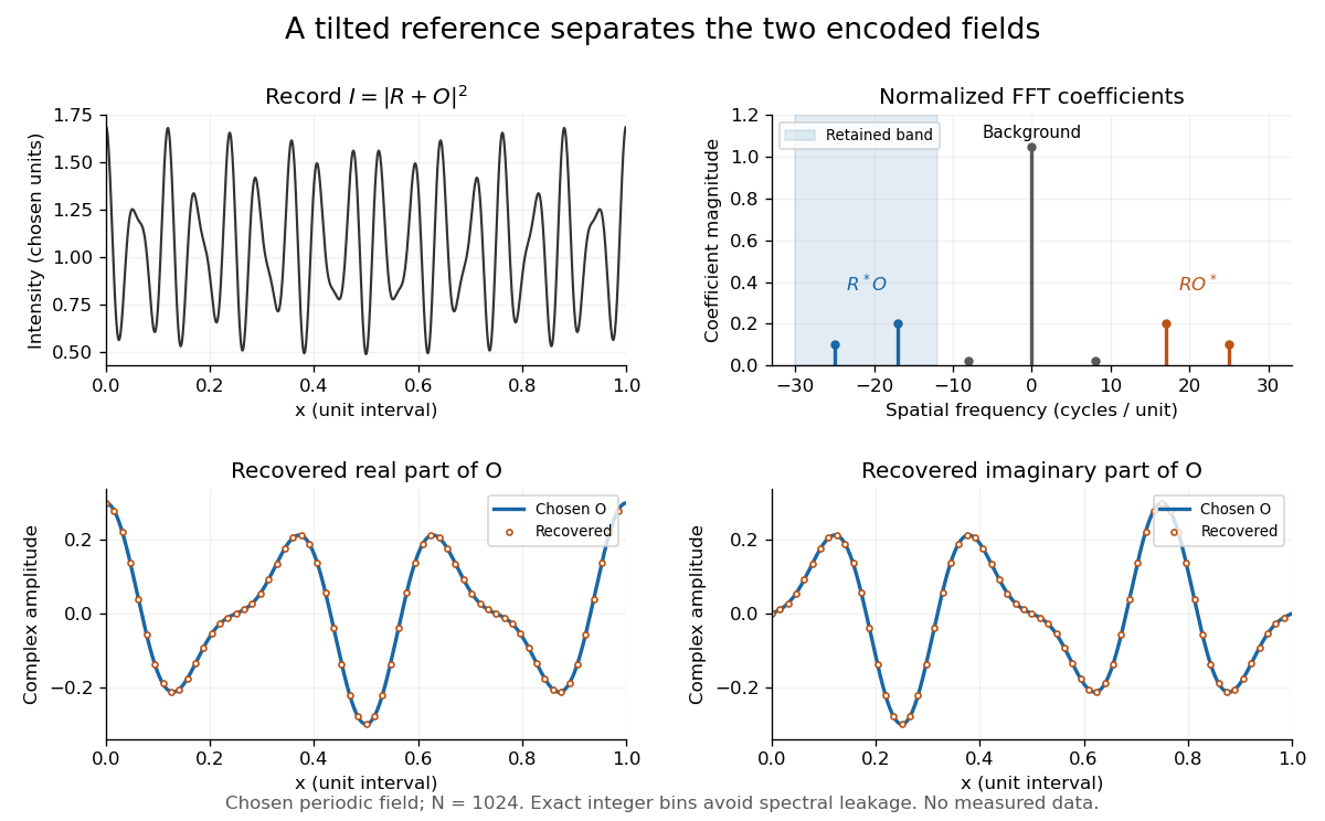
Original periodic off-axis holography calculation: separated cross terms and recovered complex amplitude
. Details. 
The figure samples equally spaced positions with the endpoint excluded, computes a normalized discrete Fourier transform using a Fast Fourier transform, retains bins , then applies the inverse discrete Fourier transform and multiplies by . The recovered real and imaginary parts coincide with the chosen to numerical precision. This exact periodic example avoids leakage by placing every frequency on an integer bin; finite nonperiodic records need allowance for broadening and an aperture.
For a continuous object field with Fourier transform confined to , the background occupies . A carrier is a sufficient separation condition for the sideband centred at , and must remain below the Nyquist spatial frequency. Here , and the Nyquist spatial frequency is . This sufficient bound describes a whole bandwidth, rather than exploiting the gaps in this particular two-component field.
The same example also makes optical playback explicit. Choose and . Since , the bounds imply , and . The affine response is stipulated; its weak-modulation interpretation is approximate. In , the desired field has frequencies ; the conjugate term has frequencies ; the background has frequencies . Thus the same carrier that separates the recorded cross terms separates the playback components. Reillumination restores a field through diffraction; computational filtering extracts the corresponding encoded field through Fourier analysis.
In-line holography 2026-10-18
In-line holography uses nearly the same direction for the holographic reference wave and holographic object wave. In a transmission geometry, the undiffracted illumination supplies while the object supplies the scattered component . This makes small optical path differences possible, but leaves the desired image, its twin image in holography and the bright background sharing an axis.
Dennis Gabor's electron-microscopy motivation led to optical tests: one line of a high-pressure mercury-vapor lamp illuminated a 3 μm pinhole, then approximately 1 mm microphotographs, recording approximately 1 cm holograms on sensitive photographic emulsions with minute-scale exposures. The roughly 0.1 mm optical coherence length favoured an in-line arrangement. Reillumination reconstructed images; focusing separated their depths incompletely. Distorted letters and random optical disturbances limited the results. These were optical demonstrations, not an operating electron microscope.[ref]
Holography, 1948-1971 by Dennis Gabor. Gabor, Holography, 1948-1971, Nobel lecture, Figs. 2–6 and accompanying optical-experiment account; authored transcription inspected at studylib.net/doc/28317456/dennis-gabor-nobel-lecture
The recorded microphotograph and its reconstructed lettering provide an object-to-image comparison in that account. The blocked-reference control described above is an explanatory control for the model; it is not a claim about an additional historical measurement.
Holographic wavefront reconstruction 2026-10-18
Take stationary scalar monochromatic waves of the same frequency and polarization of an electromagnetic wave, with time convention . Write their complex amplitudes at the recording plane as and , absorbing the common conversion to irradiance into the units. An exposure short enough to avoid fringe motion but long compared with an optical period recordsThe two cross terms are where relative wave phase enters the measured light intensity. Blocking the holographic reference wave leaves and removes them. Loss of mutual optical coherence, incompatible polarization of an electromagnetic wave or motion that averages the relative wave phase similarly reduces fringe contrast. These are useful controls for distinguishing a hologram from an ordinary brightness record. One local cosine value does not uniquely determine a wave phase; known reference structure and separation of the cross terms supply the additional information in the example below.
Model a thin weakly modulated recording by its amplitude transmittanceHere and are real constants in a local linear response to exposure at a fixed exposure time. They describe a chosen amplitude modulation model, not a universal photographic response; an absorbing negative may have . Keep for this passive real-transmission model. Ignore material thickness, saturation, shrinking, clipping and changes of wavelength. Illuminating the processed record with the original gives, immediately after the plate,This follows by multiplying the preceding identity by ; no wave phase detector has been assumed. If is uniform, the desired term reproduces up to a constant. A nonuniform weights the recovered field. With a strong holographic reference wave, the contamination is small relative to , but it is retained in this identity. Subsequent diffraction propagates each term: reproduction at the plate is the starting boundary field, not yet a focused image.
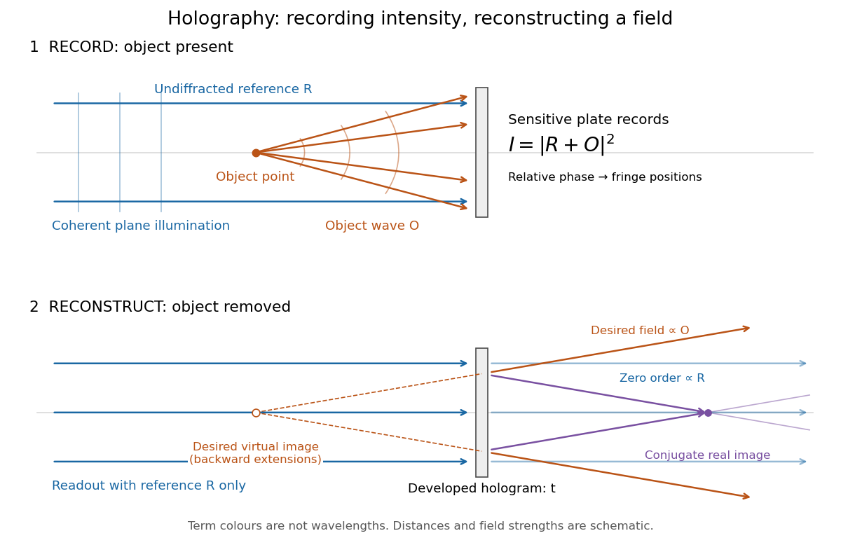
Recording light intensity and reconstructing wavefronts: original functional geometry for in-line holography
. Details. 
The schematic uses a plane wave reference and one optical point source to separate the functions. The top row records ; the bottom removes the object and illuminates the developed hologram with . Dashed extensions identify the desired virtual image; the conjugate component converges toward a real image. All three outgoing components coexist. The coloured paths distinguish terms, not different wavelengths; distances and strengths are schematic. This functional drawing is not a reconstruction of the historical apparatus.
There are unlisted articles, also show them or only show them.