
Galton's stature regression 2026-10-14
Francis Galton's paper Regression towards mediocrity in hereditary stature by Francis Galton analyzes adult offspring heights against the average of their parents' adjusted heights. He multiplied female heights by before making that parental average. Table I contains 928 adult offspring from 205 parental pairs; the opening prose instead states 930. Its grouped readout is a median, and the explanation of Plate IX describes a smoothed offspring deviation about two-thirds of the parental deviation.[ref]
Regression towards mediocrity in hereditary stature by Francis Galton. Printed pp. 247-248, Table I; pp. 261-262, explanation of Plate IX(a): adjusted heights, counts, grouped medians and 2:3 deviation ratio
These were parent-offspring records, not repeat readings of an unchanged signal. The paper's group tendency does not say that every child must be closer to the population mean. Galton also reports uncertainty over whether some recorded heights included shoes, a concrete measurement error limitation.[ref]
Regression towards mediocrity in hereditary stature by Francis Galton. Printed p. 252: shoes-on versus shoes-off uncertainty and the average two-thirds height-deviation claim
The Pearson correlation coefficient and all generated values above are our chosen model, not a reconstruction of his data.For causal inference, a before-and-after change among units selected by an extreme baseline reading combines any causal effect with the change expected from selection. In the synthetic model the selected-group mean falls by about with no intervention at all. Calling that entire fall an intervention effect would attribute a predictable measurement error contribution to a change in the signal.
One comparison design selects all eligible units by the same rule, then uses randomization to assign an intervention or a comparison condition, with the same measurement times and instrument in both groups. To see the principle algebraically, let assignment be independent of within the selected population, and let the intervention add a constant to the second reading: . ThenSubtracting the two expected changes isolates under these assumptions. Both groups experience the same selection tendency in expectation. A finite experiment still has sampling uncertainty; randomization does not guarantee identical realized groups. Without randomization, the same threshold alone does not establish comparable latent signals or error processes. Different selection rules, selective follow-up, changing instruments, or common temporal changes also require explicit assumptions. This is a statistical inference principle about comparisons, not evidence that any particular intervention works.
Repeated-measurement latent signal model 2026-10-14
Imagine an instrument measuring the same fixed quantity twice on each unit. Across units the persistent signal is a latent variable; the two measurement errors are fresh, mutually independent random variables, also independent of . Assume they have mean zero and common finite variance , while has mean and variance . ThenThus the Pearson correlation coefficient is when . Both measurements retain the same marginal mean and variance. Repetition does not make the entire population collapse toward ; it changes what we expect after selecting on .
For , further assuming normal distributions for and both measurement errors gives the conditional expectationSince , this predicted reading is closer to than is. Independence and zero mean errors alone do not justify this linear conditional expectation: without the normal distribution assumption the same expression is the linear least-squares projection, and the actual conditional expectation can be nonlinear. Correlated errors, a changing signal, or different error variances require their own model; a noisy reading by itself supplies no universal shrinkage factor.
Use a slit light source, a rectangular transparent block on plain paper, pencil, ruler and protractor. Trace the block outline, keep it fixed, and mark widely separated points on incident and emergent light rays. Remove the block and join the entry and exit points to reconstruct its internal light ray. Draw the surface normal vector at entry; measure outside and inside from that normal line. Choose a path exiting the opposite parallel face rather than a side edge. Repeat for a range of with the same block and source colour; record and repeat-reading spread. Plot vertically against horizontally: Snell's law predicts slope , approximately the block's refractive index. The emergent light ray should be parallel to the incident one. Beam width, pencil marks, protractor resolution, block movement and colour spread limit precision; a narrow-colour source reduces spread from optical dispersion. These are measured angular readings, not a direct timing of phase velocity.[ref]
A normal incidence trial checks the drawn normal and the absence of bending, but the ratio is then . Small nonzero angles also make that ratio sensitive to reading errors. Compare several trials through the slope rather than relying on one nearly axial pair. This rectangular-block measurement complements the existing total internal reflection experiment, which probes a different boundary condition.
Apparent depth 2026-10-14
A submerged object looks shallower because its emerging light rays bend away from the surface normal vector. Their backward extensions give an approximate virtual image nearer the surface. For an object at perpendicular depth in a medium of refractive index , viewed through a flat boundary from a medium of refractive index , the near-normal paraxial approximation gives . Thus the model water depth appears approximately from air. This is a bundle-of-light rays statement, not a deflection of the axial light ray.[ref]
For general transmitted light rays, specify what “depth” means. Put the object at below a horizontal boundary . A light ray reaches the boundary at , with object-side angle and observer-side angle , both measured from the upward normal vector. For , its backward extension meets the object's normal line at , whereThis axis-intercept depth is exact for that one transmitted light ray in the stated model. It tends to as the angles tend to zero; at exactly zero the quotient is interpreted as a limit. These elementary tangent, sine and cosine relations show precisely where the small-angle approximation enters.
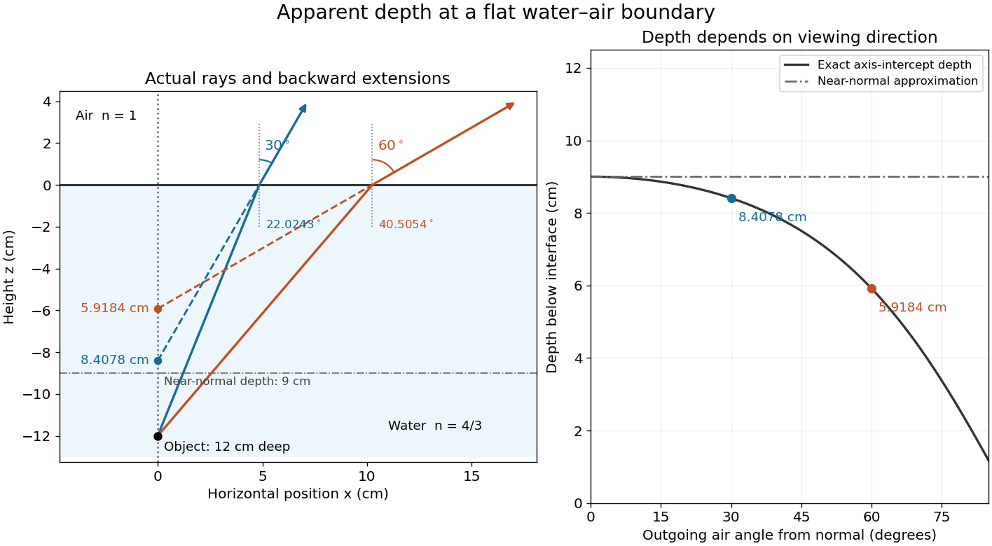
Exact light ray extensions and the near-normal apparent-depth approximation
. Original model of an object below a planar water–air boundary, with refractive indices and . The left panel has equal coordinate scales; solid lines are forward light rays and dashed lines are backward extensions to the object's normal line. The two outgoing light rays are different viewing directions, not a bundle entering one eye. The right panel compares their exact axis-intercept depths with the near-normal value . Marked points are calculated predictions, not observations. Details.
At appreciable obliquity these depths differ, so the full outgoing bundle has no single exact virtual image on the object's normal line. An oblique eye samples a narrow bundle; its local apparent position also depends on that bundle and cannot be inferred by declaring to be a universal image depth. A plane refracting boundary gives approximate image formation near normal incidence, with departures at larger angles. The construction assumes a flat surface, uniform transparent media with isotropy, and a propagating transmitted light ray; it does not extend to total internal reflection.
Interface phase matching 2026-10-14
At a stationary, uniform planar boundary, incident and transmitted plane waves have the same variation of wave phase along the interface and in time. The figure marks places where equal-wave phase wavefronts meet the boundary. Although their perpendicular spacing differs, their intersections must advance along the boundary together. This is the local mechanism behind Snell's law.[ref]
Laws of Geometric Optics. equations 946–950: common angular frequency and matching tangential wavevector components
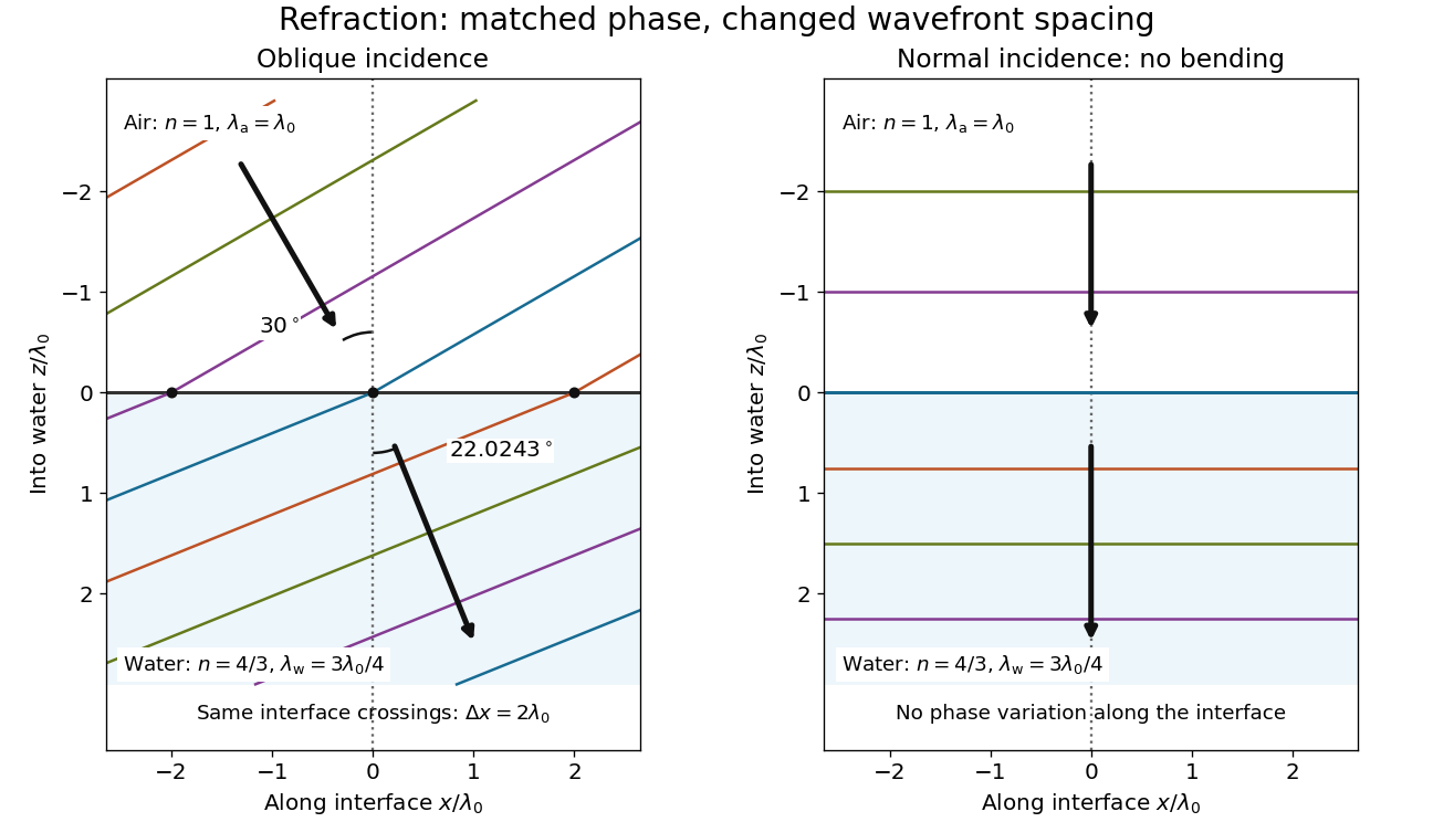
Wavefront spacing changes while interface wave phase matches
. Original plane wave construction for , and air incidence . Both panels have equal horizontal and vertical coordinate scales in units of vacuum wavelength . Coloured lines join at identical interface crossings; arrows show propagation perpendicular to each wavefront. The reflected branch is omitted. At normal incidence, the wavefronts stay parallel to the boundary and only their spacing changes. Details.
For a short derivation, let run along the interface and increase into the transmitted medium. Write each wave phase as . The electromagnetic boundary conditions must hold at every on ; their matching requires and . Constant offsets and wave amplitudes are determined separately. Since , this givesFor nonzero tangential wavenumber, the spacing of equal-wave phase intersections along the interface is . It is not the perpendicular wavelength. At normal incidence, the tangential wavenumber vanishes and the interface is uniform in wave phase.[ref]
Normal incidence 2026-10-14
At normal incidence, the incident light ray follows the surface normal vector. Snell's law gives for positive refractive indices, so the transmitted light ray does not bend. Nevertheless, its phase velocity and wavelength change if the refractive index changes. A single axial light ray therefore cannot measure apparent depth: neighboring light rays and their directions supply that information. A reflected component can still be present; no bending of the transmitted light ray does not imply complete transmission.
Angle of refraction Created 2026-10-14 Updated 2026-10-25
The angle of refraction is the angle between the transmitted light ray and the surface normal vector, measured on the transmitted side. With positive refractive indices, a propagating transmitted light ray satisfies in Snell's law. The incident and transmitted angles are measured from the same normal line, not from the surface and not from the emergent light ray at a second surface.
Angle of incidence Created 2026-10-14 Updated 2026-10-18
The angle of incidence is the angle between the incident light ray and the line of the surface normal vector at the point of incidence. Use the acute angle on the incident side, with for a nongrazing incident light ray. An angle measured from the surface itself is its complement . The same convention applies to wavevectors in the transparent media with isotropy considered here.
Work by Refael Hassin 2026-10-14
Finite-time rate-zonal separation 2026-10-14
Consider two dilute populations of spheres with the same buoyant density and radii and . Adopt the fixed linear density gradient and constant local centrifugal acceleration of linear-gradient isopycnic focusing, with constant dynamic viscosity and negligible diffusion. Stokes's law makes proportional to , so doubling radius multiplies the migration rate parameter by four, although the mass increases eightfold.
Use , and . The liquid occupies , so the matching density position lies beyond its outer boundary. Both populations begin at ; choose and . Their band-center trajectories areAt , they lie at approximately and ; at , at and . Equal buoyant density has not prevented a useful finite-time separation. Solving using the natural logarithm gives first boundary arrival at . The corresponding arrival for A is . Trajectories describe migration only until contact with the boundary; subsequent collection into a centrifugation pellet is not represented by extending the curve beyond .
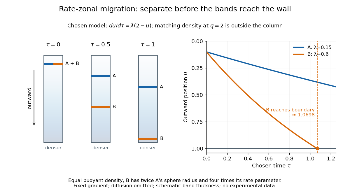

This is the useful contrast with isopycnic centrifugation: stopping time helps determine the recovered positions in rate-zonal centrifugation, whereas a stationary matching density position sets the limiting band center in isopycnic centrifugation. Real resolution also depends on initial zone width, diffusion and variations in particle properties; distinct calculated centers alone do not prove that fractions will be pure.
Transmittance 2026-10-14
Transmittance is the fraction of incident radiant flux transmitted through a specified object or boundary. Specify wavelength, angle of incidence, electromagnetic polarization and which outgoing light is collected.
Radiometric absorptance 2026-10-14
Radiometric absorptance is the fraction of incident radiant flux converted to heat in the specified receiver: , with for a passive receiver. Specify the entrance boundary, wavelength, incidence angle and receiver temperature. Radiation reflected or transmitted out of that receiver is not absorbed power. A cavity can improve radiometric absorptance by giving light repeated opportunities for wave absorption; a dark coating alone does not establish .
For broadband light, spectral radiant flux matters: . A single effective radiometric absorptance therefore depends on the incident optical spectrum as well as on the receiver. If the stated incident boundary lies before a window of known power transmission , the receiver absorbs when other optical losses are absent. Window loss and receiver radiometric absorptance are separate corrections.
Reflectance Created 2026-10-14 Updated 2026-10-18
The fraction of incident radiant flux returned by reflection, for specified wavelength, angle of incidence and collection directions.
Work by R. S. DaBell 2026-10-14
Polymerase chain reaction history 2026-10-14
The 1993 Nobel chemistry announcement credits Kary Mullis with inventing the polymerase chain reaction method and states that the technique was first presented in 1985. The reusable-product principle explains its power: each successfully copied interval can help specify the next generation. The award attribution is a historical claim; it does not imply that every improvement in DNA polymerases, thermal cyclers or PCR controls came from one person.[ref]
Press release: The 1993 Nobel Prize in Chemistry by Royal Swedish Academy of Sciences. 13 October 1993 announcement, award citation and introductory account of PCR first presented in 1985
Real-time polymerase chain reaction 2026-10-14
Real-time polymerase chain reaction monitors fluorescence during cycling. With validated specificity, calibration and PCR efficiency, that record supports estimating initial template amount; this quantitative use is called qPCR. Ordinary endpoint PCR amplification examines accumulated product afterwards. qPCR need not start from RNA, and RT-PCR need not monitor fluorescence. Combining both operations gives RT-qPCR.[ref]
Real-Time PCR (qPCR) Basics by Thermo Fisher Scientific. Real-Time PCR Basics: amplification monitoring and quantification
RT-PCR combines reverse transcription with PCR amplification. The RT names the RNA-to-DNA step, not real-time observation. RT-PCR can have an endpoint readout. A matched preparation omitting reverse transcriptase tests whether contaminating DNA could account for amplification; it answers a different question from a no-template reaction.[ref]
Basic Principles of RT-qPCR by Thermo Fisher Scientific. One-step vs. Two-step RT-qPCR and Controls for RT-qPCR: minus-reverse-transcription control
PV92 teaching experiment 2026-10-14
The DNA Learning Center's Detection of an Alu Insertion Polymorphism by PCR by DNA Learning Center, Cold Spring Harbor Laboratory supplies a concrete length-based example. It collects mouthwash biological cells, concentrates them with a microcentrifuge, heats them by Chelex extraction and transfers the DNA-containing supernatant. Its reaction combines of that preparation with primer mix and a reagent bead in a thermal cycler. Thirty cycles use , and , each for thirty seconds. An electrophoresis chamber separates products by agarose gel electrophoresis in a 2 percent gel; a UV transilluminator reveals stained DNA.[ref]
Detection of an Alu Insertion Polymorphism by PCR by DNA Learning Center, Cold Spring Harbor Laboratory. pp. 2–3, Procedures I–III: extraction, 25 microlitre reaction, cycle profile, gel and UV readout
Its PCR primers flank an insertion site at the PV92 locus. The student protocol predicts a 715-base pair product with the Alu element and a 415-base pair product without it. Two bands support a heterozygous genotype; one corresponding band supports a homozygous genotype only if amplification and detection of both alleles were adequate. These are the protocol's expected readouts, not newly collected observations.[ref]
Detection of an Alu Insertion Polymorphism by PCR by DNA Learning Center, Cold Spring Harbor Laboratory. p. 1, Introduction: primer-flanked insertion and stated 715/415 bp genotype patterns
The instructor manual describes extra bands from nonspecific priming and a small diffuse primer dimer band. A missing target band therefore cannot on its own distinguish failed extraction, inhibited copying, poor binding or lack of the target. Nor does detection of the Alu element at this one genetic locus establish a complete genome, a unique personal identity or a clinical conclusion. The PCR controls help separate these possibilities; DNA sequencing can add sequence evidence to the size comparison.[ref]
Using an Alu Insertion Polymorphism to Study Human Populations by Dolan DNA Learning Center, Cold Spring Harbor Laboratory. printed pp. 18 and 29, Results and Discussion and Amplify DNA by PCR: primer dimer and nonspecific priming
PCR specificity 2026-10-14
PCR specificity concerns whether the accumulated amplicon comes from the intended interval. Binding temperature, PCR primer nucleotide sequences and their possible alternative binding sites matter. Too permissive binding can support competing products; excessively restrictive binding can prevent the intended product. A band of the expected length is useful evidence, but unrelated nucleotide sequences can have the same length. DNA sequencing tests identity more directly, subject to mixtures and copying errors.[ref]
How to Design a Primer by Addgene. Primer Design for PCR: specificity, paired melting temperatures and complementary primer sequences
There are unlisted articles, also show them or only show them.