
Sample mean sufficiency depends on the model 2026-10-14
For the normal sample sum with known variance, assume independent and identically distributed with fixed known variance . The joint probability density factors asThe Fisher-Neyman factorization theorem proves that the sum, and hence the sample mean, is a sufficient statistic for . Its remaining deviations have a joint Gaussian law independent of and are independent of . If both and are unknown, the sample mean alone loses information about variance; the pair is sufficient for the full statistical parameter.
A discrete counterexample shows why a sample mean is not automatically sufficient for arbitrary statistical models. Let be independent and identically distributed on withEach observation has mean one. The arrangements all give sample mean one, yetThis conditional probability is at and at . The conditional distribution therefore still depends on the unknown statistical parameter: this sample mean is not a sufficient statistic. The useful reduction depends on the family of full-data laws, even when its mean stays fixed.
A sufficient statistic allows the observed likelihood function to be stored through a shorter record, up to a parameter-independent factor. For the Bernoulli sample sum as a sufficient statistic, writeThe second likelihood function belongs to the observed count; the first belongs to the observed sequence. Their absolute values differ by the binomial coefficient, but their likelihood ratios between any two interior parameter values agree. A maximum-likelihood estimator can therefore use just .
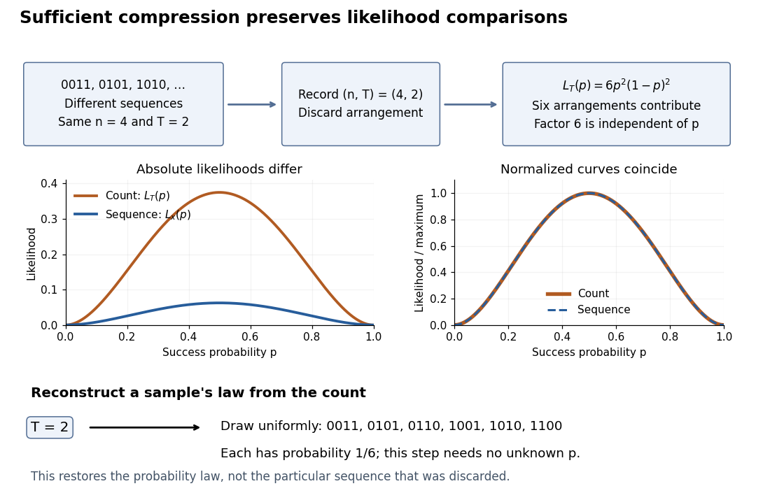
Sequence to count: sufficient compression preserves likelihood comparisons
. For , three example sequences share . Recording produces the count likelihood . Normalizing each curve by its maximum makes the two curves coincide. A reverse random draw from the six arrangements restores the full-data probability distribution, using no unknown . Details.
This compression discards which arrangement actually occurred. To reproduce the original experiment's probability distribution, first draw from its binomial distribution and then draw uniformly from the arrangements with that sum. The second step is independent of , so it supplies no additional evidence about . It does not recover the particular discarded sequence. If the scientific question changes to time trends or statistical dependence between observations, the common- independent and identically distributed Bernoulli model may no longer apply, and the ordering can become informative.
Let be fixed and known, and let be independent and identically distributed Bernoulli random variables with common success probability . Their joint probability mass function, on the binary sample space , isThere are arrangements with successes, so has the binomial distribution. For and , its exact conditional full-data probability mass function isThis conditional distribution is uniform over arrangements, with no dependence on : the sum is a sufficient statistic. [ref]
Sufficiency (Stat 210a, Fall 2025) by Will Fithian. Sufficiency, Will Fithian, “Independent Bernoulli sequence”: conditional pmf
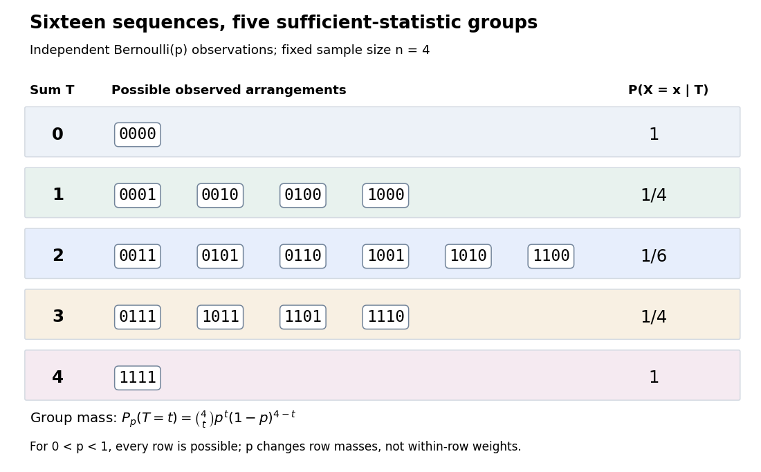
Four Bernoulli observations grouped by their sufficient sum
. All sixteen binary sequences are grouped by . Within each group the conditional distribution is uniform; changing changes the group's total probability, not the conditional weights within it. Details.
For , the group sizes are and the within-group conditional probabilities are respectively . For example, leaves exactly , each with conditional probability . At , each such sequence has unconditional probability and the group has probability . At , these values are and ; at they return to and . The conditional weights stay in all three cases.
At the boundary , only has positive probability; at , only does. Dividing by on the other groups would divide by zero. Nevertheless, the same uniform-on-arrangements Markov kernel is a valid common version for the entire family : it gives the correct point mass on the one observed group at each boundary and assigns permissible versions on its unobserved groups. Define the joint probability mass function there by the original product of the one-trial Bernoulli probability mass functions, or use the limiting convention in the compact formula.
The sample mean is an unbiased estimator of and retains the sufficient statistic because is known. By contrast, is also an unbiased estimator of but, for , is not sufficient: the conditional success probability of the independent given is still . Thus unbiasedness does not imply sufficiency.
Sufficiency also does not imply completeness of a statistic. For , the full-data sufficient statistic admits the nonzero function with expectation zero for every . Nor does minimality imply completeness of a statistic: for and the restricted statistical model , is a minimal sufficient statistic since the likelihood ratio distinguishes its three values. Yet has expectation at both parameter values and is never zero. Changing the parameter family can change completeness of a statistic even while preserving sufficiency.
Work by Steven G. Krantz 2026-10-14
Work by Steven Chu 2026-10-14
Work by Sterling Brown Hendricks 2026-10-14
List of statisticians 2026-10-14
Spreadsheet cell reference 2026-10-14
A spreadsheet cell reference identifies the spreadsheet cell read by a spreadsheet formula. In A1 notation,
B3 combines a column letter with a row number. For copying, the column and row can each be relative or absolute, independently: a $ immediately before a coordinate fixes that coordinate during the copy. The $ is an addressing marker, not a currency symbol. [ref]Switch between relative, absolute, and mixed references, Microsoft Support. Switch between relative, absolute, and mixed references: opening paragraphs and table of reference changes when copying two cells down and two cells right
Number columns as , , and so on. If a spreadsheet formula moves by columns and rows during copying, a referenced coordinate becomeswhere each is for a relative coordinate and for an absolute coordinate. This is a translation on the unfixed coordinates. For ordinary in-sheet references whose translated addresses exist, repeated copies compose by addition of their displacements: substitute the rule twice to obtain , and likewise for the row. Copying therefore preserves either a fixed coordinate or an offset from the formula's location.
Meniscus (liquid surface) 2026-10-14
Precipitation after equal-volume mixing 2026-10-14
Consider an original toy AB salt model with stipulated at fixed temperature and fixed activity coefficient product. This is a conditional concentration constant, not measured data for calcium carbonate or any identified material. A stock contains A cations and X anions; another contains Y cations and B anions. All four ions have unit electric charge magnitude. Only AB can form a solid; X and Y remain spectator ions. Assume full dissociation, no other chemical reactions, and a mixed volume equal to the sum of the initial volumes.
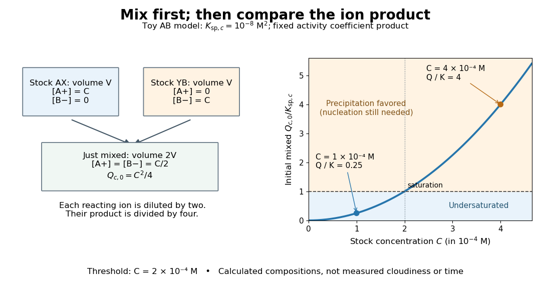
Mix two stocks, each of volume ,, each at molar concentration of its indicated salt. Before any precipitation, the mixed volume is , soMultiplying the two stock concentrations would overestimate the mixed ion product by a factor of four. The saturation threshold is .
If , mixing gives : no AB precipitate is favored. If , mixing gives . Suppose nucleation occurs and bulk AB solid remains at chemical equilibrium. Equal starting inventories and one-to-one stoichiometry require equal remaining concentrations, henceFor two portions in the second case, each reacting ion starts with ; the final chemical solution retains of each, and of AB enters the solid. The respective X and Y inventories stay at . Exactly half of each reacting inventory precipitates in this toy model.

The chemical equilibrium calculation adds a phase constraint to the inventory balance. Write and . In the equilibrated bulk model,When , the last condition requires saturation; when , the inventory can leave an undersaturated chemical solution. Together these give . This excludes a persistent supersaturated solution by its explicit chemical equilibrium assumption; it does not model a nucleation delay.
Saturation criterion for precipitation 2026-10-14
Relative to the specified solid, favors dissolution if that solid is available; favors precipitation; equality marks saturation. These comparisons identify a driving direction favored by thermodynamics, not a reaction rate.[ref]
15.1 Precipitation and Dissolution. Chemistry 2e, §15.1, Predicting Precipitation: unsaturated, saturated and supersaturated cases
A proof outline comes from the reaction Gibbs free energy for dissolution:Here is the molar gas constant and the absolute temperature. If , the logarithm is positive, making the reverse transfer into solid favorable. At equality the bulk driving difference vanishes. Equality can also occur at the boundary where the last solid disappears, but it is not a universal constraint on every solid-free chemical solution.
Ion product Created 2026-10-14 Updated 2026-10-18
The ion product evaluates the same dissolved-ion thermodynamic activity product as the solubility product, but at the current composition rather than necessarily at chemical equilibrium. For AB, ; its concentration counterpart is . Compare with only under compatible activity coefficient assumptions.[ref]
15.1 Precipitation and Dissolution. Chemistry 2e, §15.1, Predicting Precipitation: comparison of reaction quotient and solubility product
For other stoichiometries, use the dissolution coefficients as powers: gives . A solubility product is not itself the molar concentration dissolved; even in the ideal AB model in pure water, that concentration is .
SEC light-scattering detection 2026-10-14
SEC light-scattering detection adds information from scattering of light to the separation. Static scattering with a concentration readout can infer a weight-average molar mass for material in an eluting slice without the standard-family retention calibration. Dynamic scattering estimates a diffusion coefficient and hence a hydrodynamic radius. “Absolute” here means independent of a retention-to-molar mass standard curve; it still needs calibrated detectors, optical response parameters, and a valid sample model. Coeluting species produce a mixture-weighted result, rather than individually identified molecules.
A concrete manufacturer test used a Bio SEC-3 column, with particles, an Agilent 1260 Infinity G5611A quaternary pump and G5667A autosampler, a diode-array flow cell, and dual-angle/dynamic scattering detectors. A buffer solution at pH flowed at ; column and scattering detector were at . Absorbance at supplied a concentration-sensitive readout. Dilution and loading comparisons tested response: seventeen ovalbumin injections spanning – gave a reported average with relative standard deviation. The note reports poorer separation of thyroglobulin from aggregates and an elevated mass estimate, illustrating the coelution limit. Its sample filtration also limits interpretation of larger protein aggregation products removed before injection.[ref]
Determination of Protein Molecular Weight and Size Using the Agilent 1260 Infinity Multi-Detector Bio-SEC Solution with Advanced Light Scattering Detection by Sonja Schneider. Sonja Schneider, Determination of Protein Molecular Weight and Size Using the Agilent 1260 Infinity Multi-Detector Bio-SEC Solution with Advanced Light Scattering Detection, 5991-3955EN, printed pp. 2–4: apparatus, Table 1, Figure 2 and Table 3
SEC chromatogram 2026-10-14
A SEC chromatogram plots a detector signal against elapsed time or elution volume. At constant volumetric flow rate , the volume delivered after injection is ; subtraction of extra-column transport volume is needed for a column-only . Real peak widths include injection volume, column dispersion, and tubing/detector spreading. Peak position, width, and area answer different questions.
SEC molar mass calibration 2026-10-14
SEC molar mass calibration measures standards under the same column, solvent, and temperature conditions as the unknown. Over a suitable fractionation interval, a common empirical approximation iswhere specifies the molar mass unit and has inverse-volume units. Interpolation is conditional on the standards' size–molar mass relationship. SEC measures access associated with hydrodynamic size, so a branched polymer, an extended chain, and a compact protein need not share that relationship.
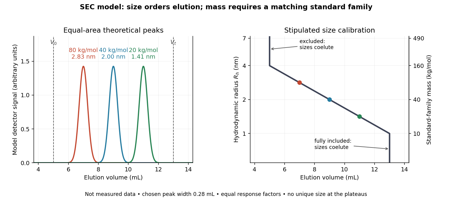

In this model the , , and standards have hydrodynamic radii , , and and elute at , , and . An unknown at would be assigned by this calibration. But a species that expands from to elutes at and is assigned without gaining any mass. The numbers demonstrate ambiguity, rather than predict a real unfolding transition.
Changes in conformational isomerism, protein folding, protein denaturation, and protein aggregation can therefore shift peaks. Association usually increases size; compaction can reduce size at unchanged molar mass. Adsorption creates a different ambiguity: delayed elution need not indicate a smaller species. A different solvent can change both polymer coil dimensions and interactions with the packing. The SEC protein conformation experiment tests these alternatives with additional detectors.
SEC fractionation range 2026-10-14
The SEC fractionation range has differential SEC pore access. Larger excluded species share ; fully included species share . Neither group can be size-ranked by elution. A broader pore distribution can trade separation per size increment for range.[ref]
Size Exclusion Chromatography: Principles and Methods by GE Healthcare. GE Healthcare, Size Exclusion Chromatography: Principles and Methods, printed pp. 17–18, Figures 1.9–1.10: selectivity curves, fractionation and exclusion limits
SEC partition coefficient 2026-10-14
For ideal SEC, define the SEC partition coefficient byHere averages solute concentration over all pore liquid, including inaccessible regions. is column elution volume. Pure steric exclusion gives ; the endpoints mean exclusion and full access.[ref]
Size Exclusion Chromatography: Principles and Methods by GE Healthcare. GE Healthcare, Size Exclusion Chromatography: Principles and Methods, printed pp. 15–16: concentration-ratio definition and Kd limits
A storage argument explains the relation. Assume a dilute stable solute, unchanged packing and solvent, constant volumetric flow rate , rapid local chemical equilibrium between pore liquid and interparticle liquid, negligible binding, and negligible transport through the pores by bulk flow. At interparticle concentration , the column holds an amount of substance . Its exit transports per unit time. The ratio is the mean residence time in this equilibrium transport model; multiplying by gives . For a narrow symmetric SEC chromatogram peak, the peak maximum approximates that mean; a strongly asymmetric peak needs an explicitly stated location convention.
The handbook also uses an operational normalizationThis denominator includes solid matrix, so full access gives when . It differs from the pore-liquid SEC partition coefficient. Read each source's volume convention before comparing coefficients.[ref]
Size Exclusion Chromatography: Principles and Methods by GE Healthcare. GE Healthcare, Size Exclusion Chromatography: Principles and Methods, printed p. 16, Figure 1.8: Kav uses Vc, not Vt
SEC total accessible liquid volume 2026-10-14
The SEC total accessible liquid volume is : interparticle plus pore liquid. A fully included nonbinding tracer estimates it. Geometric bed volume instead includes solid matrix, .[ref]
Size Exclusion Chromatography: Principles and Methods by GE Healthcare. GE Healthcare, Size Exclusion Chromatography: Principles and Methods, revision 18102218 AM, printed pp. 15–16, Figure 1.7: liquid, pore and geometric volumes
SEC void volume 2026-10-14
The SEC void volume is the interparticle liquid volume, operationally measured by a sufficiently large excluded, nonbinding tracer. It excludes pore liquid. Choose a tracer that does not undergo adsorption or change the packing; correct the measured elution for tubing and detector delay before identifying it with a column-only .
SEC pore access Created 2026-10-14 Updated 2026-10-20
In ideal SEC pore access, geometric exclusion changes the fraction of pore liquid a solute can occupy. Diffusion permits entry into and exit from accessible pores; the through-flow chiefly transports the sample between packing particles. A hydrodynamic radius is a useful size descriptor, but actual pore entry also depends on shape and pore geometry. A flexible polymer coil is not a rigid ball with a perfectly sharp entry diameter.
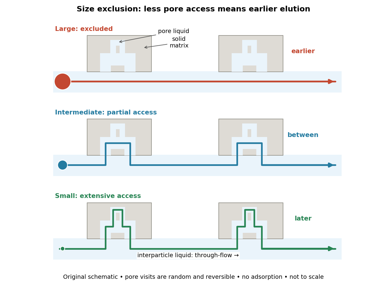

The extra delay is best understood as extra accessible storage, rather than a prescribed longer streamline. Pore visits are reversible and random. An entirely excluded species samples the SEC void volume; a sufficiently small nonbinding species samples the SEC total accessible liquid volume. Intermediate species lie between these limits. Larger hydrodynamic size generally means earlier elution within the column's SEC fractionation range.
There are unlisted articles, also show them or only show them.