
Taq polymerase Created 2026-10-14 Updated 2026-11-05
Taq polymerase is a heat-resistant DNA polymerase used in PCR amplification. It requires a paired strand end and nucleotide substrates; heat resistance does not confer target recognition.
Foil capacitor dielectric experiment 2026-10-14
Southern Methodist University's teaching lab, Introduction to the Parallel Plate Capacitor Lab, makes the response tangible with a capacitor assembled from aluminium foil, paper and taped wire contacts. Its instructions specify approximately foil rectangles, aligned with the paper completely separating them. A multimeter in capacitance mode supplies the readout; a ruler measures plate dimensions and a micrometer measures specimen thickness. The lab replaces the paper with other sheets, including cardstock, plastic wrap and wax paper. It asks students to keep foil area and alignment consistent, measure thickness at several positions, estimate thickness uncertainty, and wait for the capacitance reading to stabilize. These are published preparation and measurement instructions, not measured results reported here.[ref]
Introduction to the Parallel Plate Capacitor Lab. Experiments 1–2, Equipment You Will Be Using, and final construction and dielectric-study instructions
The inference uses each specimen's own thickness , not just a comparison of raw meter readings. With corrected capacitance and overlapping area , the ideal estimate is . A thicker sheet can give a smaller capacitance despite larger relative permittivity. This is why changing material while letting the plate gap change does not isolate electric susceptibility by itself.
Useful additional controls are to keep leads in the same positions, use capacitance measurement calibration, repeat one sheet after the others to check drift, and repeat the assembly to assess contact reproducibility. An air-gap reference must have known spacers maintaining the same separation; removing a supporting sheet and letting the foil touch is not such a reference. Record the instrument's test frequency and measurement mode when available. A capacitance display alone does not establish negligible dielectric loss or a strictly static permittivity. These are proposed controls extending the published teaching instructions.
Air gaps produce a particularly revealing systematic error. Suppose a uniform sheet of thickness and relative permittivity is separated from the electrodes by air layers of total thickness . Approximate air permittivity by vacuum permittivity, neglect the fringing field of a capacitor and use the same area in each layer. The common normal electric displacement field has magnitude , so integrating the electric field through the layers givesIf the analyst inserts the sheet thickness alone into the ideal filled-gap formula, the inferred value isFor the stipulated model and , this gives , not three. These values are calculated examples, not measured sheet properties. If total plate separation is used instead, the effective estimate is ; it still mixes the sheet and the air. Thus measuring a thickness accurately cannot compensate for an unrecognized layer.
The fringing field of a capacitor and additive lead capacitance further limit a foil measurement. Keep lateral plate dimensions large relative to separation, and use a guard electrode of a capacitor in a suitable fixture for more demanding work.[ref]
Materials Measurement: Dielectric Materials. Solution: guarded three-electrode fixture, fringe capacitance, specimen flatness and air gaps
A family of thickness measurements can help distinguish material response from an additive offset, but air gaps can vary with the assembly. A large, repeatable reading supports a capacitance change; extracting a material electric susceptibility requires the geometry, gaps, instrument response and dielectric loss assumptions to survive these checks. No measured relative permittivity is claimed for any of the lab's sheets. Dielectric breakdown Created 2026-10-14 Updated 2026-10-20
Dielectric breakdown is failure of an insulating regime under a sufficiently strong electric field, allowing substantial electric current through the material. For example, an electron freed from a chemical atom or molecule can become a mobile charge carrier. The small-field linear electric susceptibility model does not describe this conducting state.[ref]
8.5 Molecular Model of a Dielectric. §8.5, dielectric breakdown paragraph immediately before the definition of dielectric strength
Electrical insulator 2026-10-14
An electrical insulator has sufficiently small transport of electric charge for its operating conditions. Insulation is a practical requirement involving electric potential difference, temperature, geometry and duration, rather than a universal claim of zero electrical conductivity. Electric polarization can be substantial in an electrical insulator; dielectric breakdown can end the insulating regime.
For an idealized uniform slab with small constant electrical conductivity , the Ohmic conductor model predicts leakage electrical resistance in parallel with capacitance . An isolated capacitor then hasThis is a derived model of slow discharge, not an assertion that every leakage mechanism obeys Ohm's law. Its time scale matches charge relaxation. The fixed-charge comparison in dielectric capacitor response needs an observation time short compared with , but long enough for electric polarization to settle. During a maintained voltage, leakage consumes power as Joule heating; delayed electric polarization can add dielectric loss under changing electric fields.[ref]
Materials Measurement: Dielectric Materials. Overview: real and imaginary permittivity, storage and dissipated loss
Large relative permittivity alone does not rule out either mechanism.[ref]
8.5 Molecular Model of a Dielectric. §8.5, paragraph following Table 8.1: high dielectric constant does not ensure a good insulator; mobile ions permit conduction
Dielectric capacitor response 2026-10-14
Compare two initially identical parallel-plate capacitors with plate area , fixed gap , vacuum capacitance , and initial electric potential difference . Completely fill both gaps with the same uniform linear dielectric of static relative permittivity , neglecting the fringing field of a capacitor. Keep one connected to an ideal voltage source and isolate the other. The geometric capacitance becomes in both cases; the electrical constraint determines what else changes.[ref]
8.4 Capacitor with a Dielectric. §8.4, Figure 8.17 and equation (8.11): isolated capacitor, unchanged free plate charge and increased capacitance
Write , and . Applying , and the capacitor energy formula gives the complete comparison:Thus the statement that a dielectric reduces the electric field needs the fixed-free-charge condition. With fixed electric potential difference, the voltage source supplies additional free plate electric charge, maintaining despite the new bound electric charges.
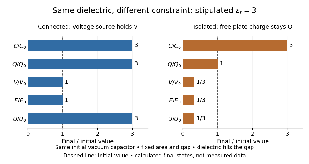
Dielectric capacitor response at fixed voltage and fixed charge
. Original normalized comparison for the stipulated model : every ratio is relative to the same initially charged vacuum capacitor. The dashed line marks the initial value. The bars show final values, not a time history or measured data. Plate geometry is unchanged and the dielectric completely fills the gap. Details.For the stipulated example, the voltage source supplies . At constant , its delivered electrical work is , whereas the increase in capacitor energy is . In an ideal reversible quasistatic insertion, the remaining is mechanical work delivered by the assembly, as accounted for in fixed-voltage capacitor energy balance. For the isolated assembly, capacitor energy falls from to , allowing of mechanical work in the same ideal limit. Actual losses reduce recoverable work; energy increases in the connected case do not arise from the dielectric supplying free energy.
Microscopic dielectric polarization 2026-10-14
Two routes to electric polarization are displacement and reorientation. An electric field can shift the centres of positive and negative electric charge in a neutral chemical atom or molecule, inducing an electric dipole moment. A polar molecule already has an electric dipole moment; a field biases its orientation. At finite temperature, random molecular motion opposes complete alignment, so a nonzero average need not mean that every electric dipole points the same way.[ref]
8.5 Molecular Model of a Dielectric. §8.5, Figures 8.19–8.20 and the thermal-fluctuation qualification following Figure 8.20
For a single species with number per unit volume , the electric polarization isThe brackets denote the local average electric dipole moment, rather than its magnitude. Opposite orientations can cancel while individual electric dipole moments remain nonzero.[ref] This averaging explains how an initially unpolarized material can respond strongly without acquiring net electric charge.
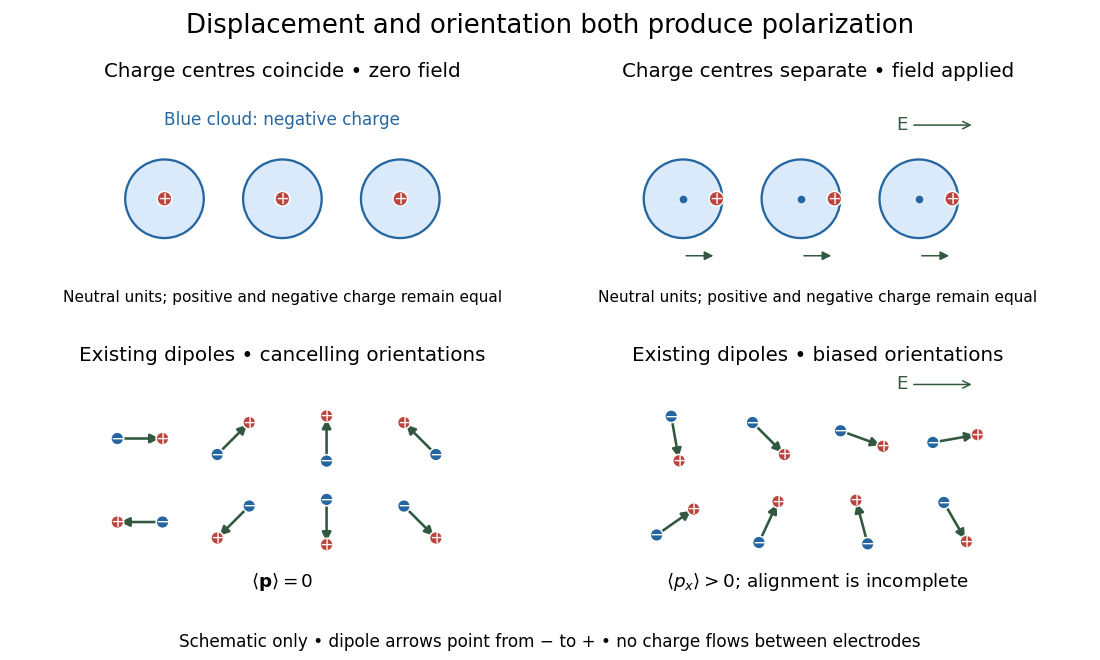
Two microscopic routes to electric polarization
. Original schematic: upper panels show coincident charge centres becoming separated; lower panels show existing electric dipoles changing from cancelling orientations to a biased distribution with incomplete alignment. Arrows run from negative to positive electric charge. Positions, displacements and orientations are illustrative, not measurements or a simulation of a particular substance. Details. Work by Dexter M. Easton 2026-10-14
Decision-tree query cost 2026-10-14
For a particular decision tree , its decision-tree query cost is the number of queries along the graph path followed by input . Its actual tree depth isThe query vertices count as operations; each is followed by one answer edge. Thus a leaf reached after queries has graph path length , and a tree consisting only of an output leaf has depth zero. With no repeated coordinates, . The decision-tree depth minimizes over all correct decision trees for ; measures the chosen algorithm, while measures the Boolean function.
Choose an input probability distribution and let have that distribution. Then is a random variable even when the decision tree is deterministic. Its probability mass function describes how often each path length occurs, and its expected value is the expected query cost. None of these quantities changes the actual maximum depth of .
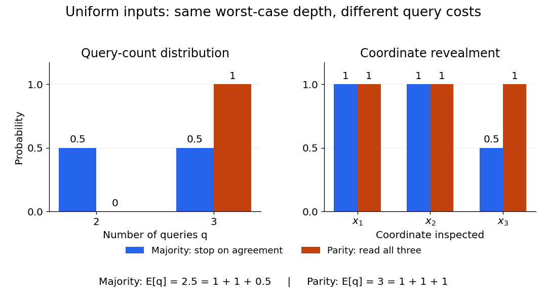
Uniform three-bit inputs: query-count distributions and coordinate revealment for majority and parity
. Details. The left panel aggregates the eight inputs from the three-bit majority decision tree: four cost two queries and four cost three. Parity always costs three. The right panel asks a different question, which coordinates are inspected: the majority function algorithm always queries coordinates 1 and 2, but queries coordinate 3 only on disagreements. These are probabilities of inspection, not probabilities that a bit equals one.
Parity lower bound for Boolean queries 2026-10-14
For three bits, the Boolean function outputs one when is odd, where denotes exclusive or. Unlike the three-bit majority decision tree, an exact decision tree computing parity must inspect all three bits on every input. If any coordinate is unread, two completions differing only at that coordinate follow the same observed graph path but have opposite parity. A single leaf cannot correctly label both.
The same argument works for bits: parity needs all queries on every input, whatever their order. Thus its decision-tree depth is , its expected query cost is for every input probability distribution, and each coordinate revealment is one. The algorithm remains required to be correct on the whole Boolean cube, even if the chosen probability distribution assigns some inputs zero probability; a promise restricting permitted inputs would be a different computational problem.
Three-bit majority decision tree Created 2026-10-14 Updated 2026-10-20
Three votes give a small but revealing majority function:Our decision tree queries , then . If these bits agree, return their common value: two equal votes already force the majority function. If they disagree, query and return its value. The first two queries have a fixed order, but whether a third query occurs is adaptive.
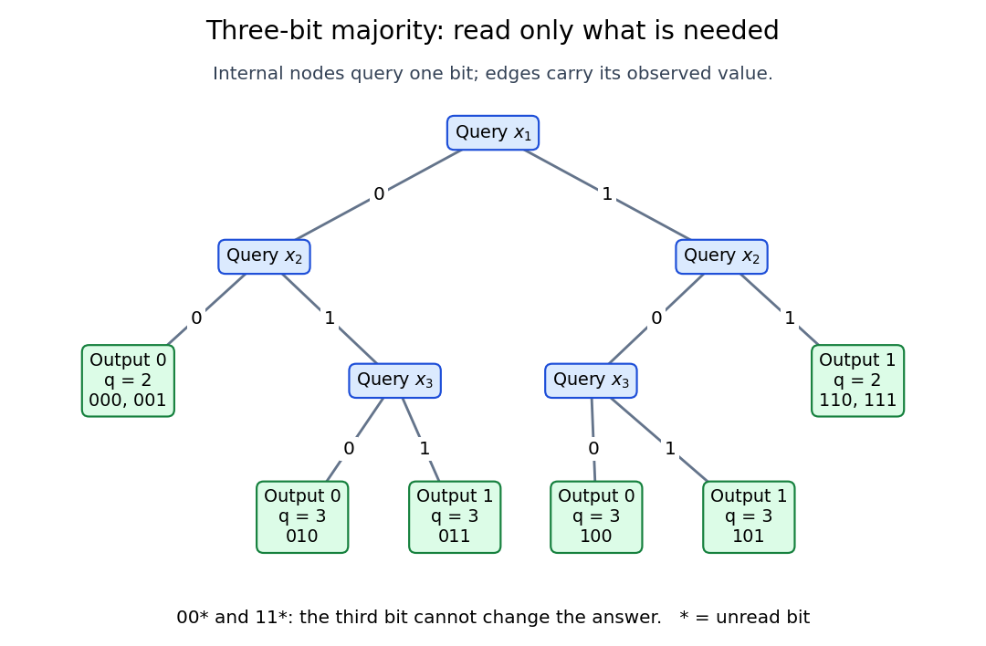


Each internal label in the diagram names the next bit to inspect. Each leaf lists its output, decision-tree query cost , and compatible inputs; an asterisk denotes an unread bit. The two shallow leaves each cover two inputs, while each deeper leaf covers one. Reading every bit would also compute the majority function, but would miss these exact shortcuts.
All eight inputs give the following exhaustive check. The parity column is the parity of , computed by exclusive or; its decision-tree query cost is justified under parity lower bound for Boolean queries.
The worst inputs for this decision tree are , exactly those with . Its actual depth is three. Every exact decision tree for this majority function has depth at least three: after the first query, an adversary can answer the second distinct query with the opposite bit, leaving the last bit decisive. Consequently its optimal decision-tree depth is , even though some inputs finish sooner. Every input has a two-bit query certificate, namely two agreeing votes; locating those votes can require a third query. This separates having a short query certificate from finding one.
Work by David P. King 2026-10-14
Work by David J. Livigni 2026-10-14
Work by David B. Bylund 2026-10-14
Work by D. R. White 2026-10-14
Pseudo-arclength continuation 2026-10-14
Pseudo-arclength continuation allows both the state and the parameter to change. Write and choose a unit vector in the kernel of the full Jacobian matrix . A continuation predictor-corrector step seeks the next solution on a hyperplane perpendicular to , a distance along the old tangent vector. This adds one equation to and makes the correction a square system. The constraint approximates arc length; is the displacement projected onto the old tangent vector, rather than the exact curved distance.[ref]
Fold of a solution branch 2026-10-14
A nondegenerate fold of a solution branch in a smooth scalar equation satisfies the displayed conditions. The implicit function theorem still gives because . Implicit differentiation gives and : the parameter has a genuine local extremum on the curve.
In the cubic polynomial, gives , and substituting into gives . Furthermore, . Yet never vanishes, so the full solution branch remains a regular level set everywhere. The obstruction belongs to the projection onto , not to the curve itself.
For systems, the cited continuation account uses a one-dimensional kernel of and outside its image of a linear map to define a simple fold (its Definition 2.2). These conditions make have full rank and support a transverse correction. A nonzero second-order term along the kernel is additionally needed to describe a nondegenerate quadratic turning point; in the scalar example this is .[ref]
Condition Estimates for Pseudo-Arclength Continuation by K. I. Dickson and others. §2.2, Definition 2.2, printed p. 265: one-dimensional kernel of the state Jacobian and parameter derivative outside its range
Parameter continuation 2026-10-14
Parameter continuation changes by a small amount and solves again for , using the previous solution as the initial guess for Newton method. If is an invertible matrix, the implicit function theorem gives a local solution branch , withLocal convergence of Newton method also needs regularity and a sufficiently small step: the cited result assumes a Lipschitz continuous derivative and an invertible at the seed.[ref]
Condition Estimates for Pseudo-Arclength Continuation by K. I. Dickson and others. §2.1, Corollary 2.1, printed pp. 264–265: Lipschitz continuously differentiable map, nonsingular state Jacobian, and a sufficiently small parameter increment
For the cubic polynomial,The derivative becomes unbounded at either continuation fold, and the scalar Newton method divides by there. Just beyond the upper continuation fold, no nearby real solution exists at the increased , although a distant negative- solution still exists. Converging to that solution would jump away from the local solution branch. Decreasing the parameter step cannot make a valid smooth local description at the bend.
Solution branch 2026-10-14
A solution branch is a portion of a solution set followed continuously as a curve. For with , a full Jacobian matrix of rank makes the nearby solution set a one-dimensional regular level set. It need not be a graph of a function : a continuation fold can obstruct that particular choice of parameter while leaving the solution branch regular.
Edge count of a complete graph 2026-10-14
For a finite set of vertices, a simple graph selects some of their unordered pairs as edges. There are ordered pairs of distinct vertices; each unordered pair is counted twice, giving possibilities. Hence every simple graph on those vertices satisfieswith equality exactly when is a complete graph. The binomial coefficient also shows why the count grows quadratically with the number of vertices.
If is an infinite set with its cofinite topology and is a Hausdorff space, every continuous map is a constant function. Otherwise two distinct image points would have disjoint open neighbourhoods. Their inverse images would be nonempty disjoint open sets of , contradicting its hyperconnected space property.
For example, from with its cofinite topology into the real line with its usual Euclidean metric is not continuous: the inverse image of the open interval is , which is not open in the infinite domain. A continuous real-valued readout on that domain can only report one value. Finite cofinite domains are different: their discrete topology allows arbitrary functions into any topological space.
There are unlisted articles, also show them or only show them.