
Every subset of a cofinite space is compact 2026-10-14
Every subset of a cofinite topological space is a compact subset. To see the finite reduction directly, take an open cover of a nonempty by open sets of and choose one member containing a point of . Since has finite complement, the set is finite. Choose a covering member for each of those remaining points. Those members together with are a finite subcover. The empty set is already compact.
Equivalently, the subspace topology on is itself cofinite: for finite , the trace of is . The argument applies again inside . A concrete open cover of needs only the two members and when these labels are distinct: each fills the other's single gap.
On , the subset of even integers is compact but not closed, because it is infinite and proper. A compact subset of a Hausdorff space is guaranteed to be closed, whereas compactness without the Hausdorff space assumption does not suffice. Changing the topology changes compactness: the same infinite set with its discrete topology has the singleton open cover, which has no finite subcover. The finite-exception argument is special to finite complements; in the cocountable topology, compact subsets of a cocountable space must instead be finite.
Sequence convergence in the cofinite topology Created 2026-10-14 Updated 2026-10-31
By convergence of a sequence in a topological space, means that every open neighbourhood of contains all sufficiently late terms. In the cofinite topology, this is equivalent to the condition that, for every , the value occurs only finitely often. Necessity uses the open neighbourhood ; sufficiency chooses an index beyond every last occurrence of the finitely many points excluded by a given open neighbourhood.
Consequently a sequence with distinct terms converges to every point of . For the original choice on , take the two open neighbourhoodsAll terms with lie in and all terms with lie in . More generally, each finite excluded set has a last visit, so and , and in fact for every . No numerical distance is tending to zero here; the open sets specify the meaning of convergence.
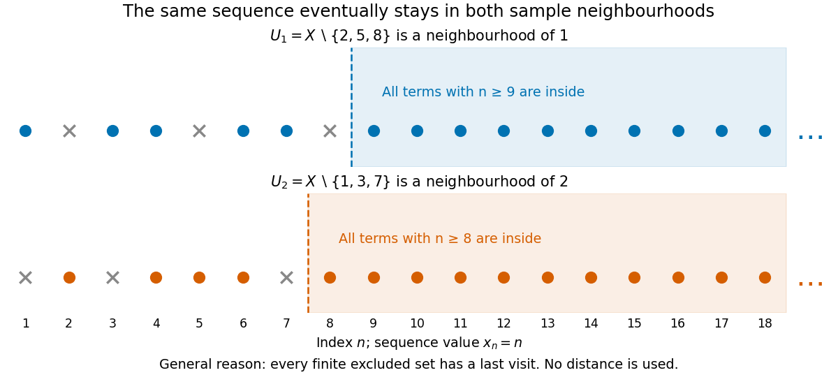
The same sequence eventually stays in neighbourhoods of two different limits
. Original sequence in the cofinite topology. Two sample neighbourhoods have different finite exclusions and different last-visit indices. Their memberships illustrate the general finite-exclusion argument; testing just these two neighbourhoods would not by itself prove convergence. Details.Distinct terms are sufficient, not necessary. The sequence also converges to every point, since each value occurs only twice. By contrast, the constant sequence converges only to : an open neighbourhood of any can exclude . The alternating sequence converges to no point, since some value different from any proposed limit occurs infinitely often.
Cartesian frame 2026-10-14
A Cartesian frame combines a chosen origin point with a Cartesian basis , including its ordering as an ordered basis. A point has coordinate vector when . The basis supplies measuring directions and unit lengths; the coordinate vector is the resulting tuple of numbers; the Cartesian frame additionally fixes where measurement starts. A vector already belongs to a vector space with a zero vector, so expressing it in a basis requires no additional choice of spatial origin.
For example, keeping the standard basis but moving the origin from to changes the coordinates of the physical point from to . This happens because is a different displacement vector. By contrast, the two diagrams above keep fixed and change only the basis. In a fixed reference Cartesian frame, a new frame with origin column and basis-column matrix describes points by ; the new coordinates are when is an orthogonal matrix.
Keep the same origin and the same vector , but use the nonperpendicular basis vectors and . They form a basis because the column matrix has nonzero determinant:The reconstruction is . Its coordinates are read along lines parallel to the other axis, producing a parallelogram. These lines need not be perpendicular to the axis being measured. In contrast, the dot products are and ; treating those as coordinates would reconstruct , a different vector.
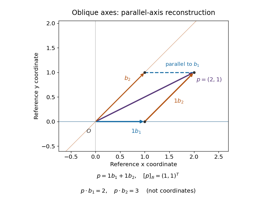
The dual basis supplies the right measuring rules for any basis.[ref]
Linear Algebra Done Right by Sheldon Axler (4th edition). §3F, Definition 3.112 and Theorem 3.114, printed p. 106: dual basis and coefficient extraction
Here these coordinate functionals are and , the rows of . They give . Equivalently, their representing vectors , satisfy and extract the coordinates as . These are Riesz dual basis in an inner product space representatives, rather than the original basis vectors.The Gram matrix records how the nonperpendicular directions interact:For any real basis represented by a square invertible matrix , writing gives these identities immediately. One can recover the coordinates either as or by solving . In this example, if , the squared norm is , not . Oblique coordinates remain useful when natural directions are not perpendicular, but the Gram matrix must accompany them when computing lengths or dot products.
Cartesian basis under rotation 2026-10-14
Rotate the standard basis through using the rotation matrix whose columns are the new basis vectors:Here and , so is an orthogonal matrix with , where denotes transpose and is the identity matrix. For the same vector , its coordinate vector in this Cartesian basis isThus and : travel forwards along and a little backwards along to reconstruct . The orthogonal projections onto the two axes give these signed coordinates because the measuring vectors are both perpendicular and of unit length.
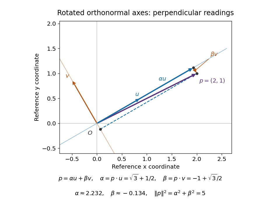


The squared norm remainsThis is useful when choosing axes aligned with a geometric feature: the coordinates change but distances and dot products retain the same sum-of-products formula. The two directions of the change of basis must be kept straight: reconstructs the vector in old coordinates, , and extracts its new coordinates. Applying to the old coordinate vector instead would actively rotate the vector.
A short proof explains both formulas. If , multiplication by gives . Then . Perpendicular unit-length columns make the matrix inverse equal the transpose; this is the computational convenience supplied by a Cartesian basis.
Work by C. D. Vaughn 2026-10-14
Work by Brian B. Hoffman 2026-10-14
Work by Boyd E. Terry 2026-10-14
Molecular dipole cancellation 2026-10-14
Molecular dipole cancellation occurs when nonzero contributions to a molecule's electric dipole moment cancel under vector addition. In a bond dipole model, use ; adding magnitudes instead discards the molecular geometry. A symmetric linear molecule with two equivalent opposed bond dipoles has and , hence zero total electric dipole moment even though each chemical bond is polarized. Carbon dioxide provides the familiar molecular example; water's bent molecular geometry permits a nonzero total.[ref]
Chemistry 2e. §7.6, Figure 7.27 and accompanying paragraphs: cancellation in carbon dioxide, noncancellation in water
For an original geometry calculation, give a fictitious three-site model a central effective electric charge at the origin and two terminal electric charges atHere is the stipulated bond length, the angle between the two connections, and is independent of any electronegativity scale. Equivalently, split the central into two colocated contributions, one for each neutral bond dipole. With , the physical electric dipole moments point from the terminal sites towards the central site:The sideways components cancel; the components along the angle bisector add. Thus . At the result is zero; at the stipulated it is exactly . This is an angle example for a model, not the measured angle or electric dipole moment of water.
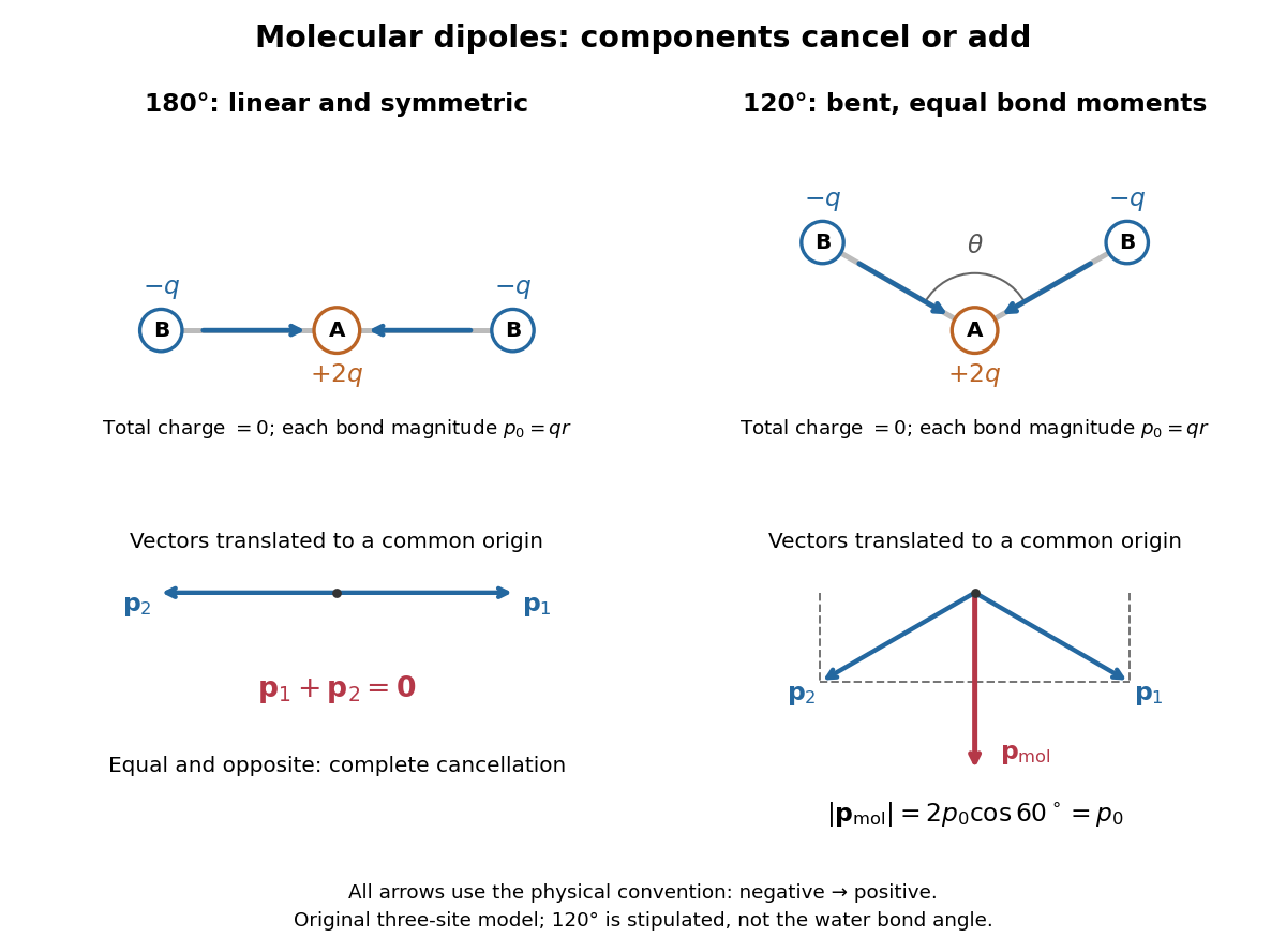
Vector addition of physical bond dipoles in a stipulated neutral three-site model: cancellation at , a bisector resultant at
. Central effective electric charge , terminal electric charges , and equal bond lengths . Arrows point from negative to positive electric charge. The lower panels translate the bond dipoles to a common origin and show their components; they are vectors, not electron trajectories or extra bonds. Details.
Opposition alone is insufficient: a linear molecule with unequal opposed bond dipoles of magnitudes and retains magnitude . Conversely, symmetry can enforce exact cancellation beyond a particular bond dipole partition. If the complete charge density invariant under point reflection about the origin satisfies , contributions to cancel in pairs. That proof uses the whole electric charge distribution, including lone pairs and atomic nuclei. It explains why molecular symmetry is stronger evidence for zero permanent electric dipole moment than a rule based only on tabulated electronegativity differences.
A permanent molecular electric dipole moment is specified relative to the molecule's orientation. An ensemble with random orientations can have zero mean laboratory vector while each molecule is polar. That orientational average differs from internal molecular dipole cancellation. The Stark effect and molecular beam electric resonance probe molecular electric dipole moments through state-dependent responses to an electric field.
Work by Billy W. Mangum 2026-10-14
Jacobi-Anger expansion Created 2026-10-14 Updated 2026-10-18
A Fourier series expansion of a sinusoidally modulated complex wave phase in Bessel functions of the first kind.
Nonpolarizing beam splitter 2026-10-14
A nonpolarizing beam splitter is designed for approximately equal power splitting ratios for the two orthogonal linear polarizations, at specified wavelengths and angle of incidence. It need not be 50:50, lossless, or have equal transmission and reflection wave phases for both linear polarizations. A scalar beam splitter scattering matrix therefore still requires a specified electromagnetic polarization and operating range. Polarizing beam splitters instead aim to separate those linear polarizations into different paths.
Coherent beam splitter recombination 2026-10-14
Suppose the two input beams share frequency, electromagnetic polarization and overlapping transverse profiles at each output, with stable relative wave phase during the photodetector's averaging interval. For the ideal beam splitter scattering matrix above, expanding the squared complex amplitudes givesThe imaginary part terms describe wave interference. Applying the single-input power split to each input separately and adding the results would discard these terms. Their opposite signs ensure : conservation of energy survives even when one output is dark.
For an original example, let , and . Then and :
| Relative input wave phase | Output power | Output power |
|---|---|---|
At , makes and ; at the dark output swaps. Thus the two inputs can feed all their combined power into one output without gain. At zero relative input wave phase, the splitter's own relative wave phase leaves the contributions in quadrature, so neither output is dark.
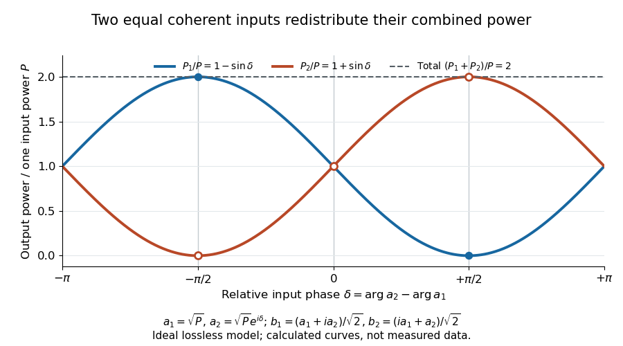
Relative input wave phase redirects the combined power of two coherent beams
. Original ideal-model curves for , and . Output powers are normalized by one input's power ; their sum is always . Markers show the three worked cases. These are calculated curves, not measured data. Details.
For fluctuating fields, average the cross term as . It vanishes for mutually uncorrelated inputs, making the independent power-splitting rule valid for the averaged output. Partial first-order optical coherence reduces it. Orthogonal linear polarizations eliminate the cross term in a polarization-insensitive power readout, and spatial mismatch reduces the overlap. Detector averaging can also erase rapid relative wave phase changes. A fixed relation between two inputs can be prepared by splitting one laser beam and recombining the two arms.
An actual teaching protocol in Michelson Interferometer & Precision Wavelength Measurement — Week 1, University of Colorado Boulder, §§4–6, starts with an ideal-model prediction, then builds a Michelson interferometer using a helium-neon laser, a nonpolarizing beam splitter, adjustable mirrors, a micrometer translation stage and a photodetector. Steering mirrors align beam overlap at near and far planes; far-plane interference fringes refine alignment. Moving the arm mirror changes the returning relative wave phase; detector voltage is watched with a live acquisition display or oscilloscope. The guide compares measured arm powers with 50:50 splitting and asks for a revised field model. It tests electromagnetic polarization dependence, optionally changing one arm with a quarter-wave plate, and estimates noise from repeated readings at fixed mirror position. These controls test whether fringe changes reflect coherent recombination rather than splitter imbalance or misalignment. The guide supplies a protocol, not a numerical dataset. Its detector noise, imperfect overlap and electromagnetic polarization mismatch limit displacement inference.[ref]
Additional background subtraction controls follow from the field model: block both arms to record the detector offset and ambient light, then unblock each arm separately to establish its detected power at fixed gain. With both open, scan the mirror and compare extrema after subtracting that background. Keep the detector below saturation and repeat the scan to check drift. A changing signal alone cannot distinguish source optical coherence from motion or changing overlap. For a vacuum round trip, a mirror displacement changes relative wave phase by ; the useful signal is its modulation after detection, not an optical-frequency oscillation that the detector must resolve.
Beam splitter scattering matrix 2026-10-14
For a linear, fixed-frequency beam splitter, choose power-normalized complex amplitudes at its input optical ports and at its output optical ports: and are powers. The scalar description treats one specified electromagnetic polarization and matching transverse profiles; other fields require additional components. With the geometrical ordering in the diagram,Here are transmission complex amplitudes per unit input and are reflection complex amplitudes per unit input. In this power normalization, a single input gives and . Raw electric field amplitudes in different media generally need additional power-normalization factors.
If these two output optical ports account for all outgoing power and the device has no loss or gain, is a unitary matrix:The dagger is the Hermitian transpose and a star is complex conjugation. To prove the condition, substitute into conservation of total power for every input vector: . Inputs and fix the diagonal entries; and fix the real and imaginary parts of the off-diagonal entry. A lossy two-output description instead has for a passive device.[ref]
Photon quantum mechanics and beam splitters by Charles H. Holbrow and others. Photon quantum mechanics and beam splitters, §IV.A, printed p. 262, equations (1)–(5): unitary beam splitter matrix and phase constraints
One consistent ideal symmetric 50:50 choice isEach reflection carries relative wave phase in this convention. The columns have unit vector norm and zero inner product, directly verifying that is a unitary matrix. Choosing a different phase convention for complex amplitudes at the optical ports replaces by , where the are diagonal matrices whose entries have modulus one; the input complex amplitudes must be transformed consistently. Observable powers are unchanged. The displayed is a convention for this ideal model, not a universal reflection rule for every coating or incidence geometry.
Optical port Created 2026-10-14 Updated 2026-10-25
An optical port specifies where and in which direction a beam enters or leaves an optical instrument. To attach one complex amplitude to it, also specify the beam's transverse field profile, electromagnetic polarization, frequency and reference plane for wave phase. Reversing propagation changes the input/output assignment. Four geometrical connections do not imply four independent input complex amplitudes in the chosen two-input configuration.
For real , defineThe integrand is positive and at most , so and the improper integral converges. Substituting also gives in terms of the exponential integral; the original representation makes positivity and the large- behavior transparent.
Apply the exact finite geometric series identity inside the integral, without assuming that an infinite series can be integrated term by term:The Gamma integral gives . Therefore, with retained terms,This remainder formula proves the asymptotic expansion at every fixed order: as . Its sign also gives alternating bounds: an odd overestimates , and an even underestimates it.
At , an independent evaluation of the integral gives . Three retained terms giveFive retained terms give with error bounded by . The actual errors are about and , respectively. The error bound is conservative, but established without relying on the numerical integral evaluation.
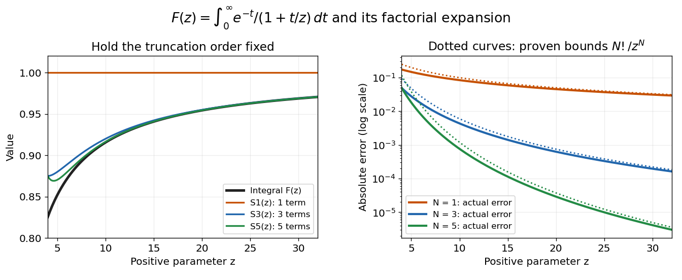

Nevertheless, the formal infinite series diverges at every fixed . The magnitudes satisfy , so they eventually increase without bound. In particular, the terms fail the necessary zero-term condition for a convergent series. The finite remainder identity remains valid after convergence has failed; this is precisely what makes the example useful.
Error bound 2026-10-14
An error bound is an established upper bound on a specified approximation error, on a stated domain and under stated assumptions. A numerical comparison at selected points can test an approximation but does not by itself establish a bound throughout that domain. An absolute error bound controls ; a relative error bound additionally specifies the reference scale.
Work by Anthony E. Butterfield 2026-10-14
Work by Anne-Marie Chang 2026-10-14
Lilium Created 2026-10-14 Updated 2026-11-05
There are unlisted articles, also show them or only show them.