Past exam of the quantum condensed matter course of the University of Cambridge 2018 Section B B4 Solution by  Codex 0 2026-10-18
Energy and momentum measurement. In angle-resolved photoemission spectroscopy, monochromatic photons illuminate a clean surface in vacuum, and an electron energy analyzer measures the outgoing kinetic energies and emission directions. Measuring both gives the occupied electronic band structure, rather than only a momentum-integrated distribution of removal energies.
Choose a common energy reference for initial and final states. Let be the initial electron energy, the Fermi energy, and the vacuum level immediately outside the sample. The binding energy is . For a direct emission event without additional losses, conservation of energy givesHere the work function is the energy from the Fermi level to the local vacuum. The initial and final energies are total single-electron energies on the same scale, while is measured above vacuum. The diagram illustrates each interval independently.
Neglecting ultraviolet photon momentum, photoemission momentum conversion giveswhere is measured from the surface normal. Parallel crystal momentum is conserved modulo a surface reciprocal lattice vector; the surface breaks perpendicular translation symmetry. A three-dimensional sample therefore generally needs a final-state model to infer perpendicular momentum. The stated two-dimensional sheet avoids that ambiguity. The kinetic energy used in this formula is the sample-vacuum value; if the analyzer and sample have different work functions, their contact potential must be included when converting the analyzer's reading, as in photoelectron binding energy reference.
Spectral information. Define and the electron spectral function by . In the sudden approximation, the basic photoemission intensity and spectral function relation isbefore instrumental broadening and background are included. Here is the Fermi-Dirac distribution, and is the transition matrix element. The electron removal spectral function contains the occupied part of the spectrum. In a noninteracting band it has a delta peak at the band energy; interactions shift and broaden peaks and can add incoherent weight. Thus peak trajectories reveal dispersion, while line shapes can constrain lifetimes after resolution effects are accounted for. Dividing by known matrix and occupation factors can estimate where those factors are appreciable; intensity alone is not identical to , and a missing peak can reflect a matrix-element suppression. States well above are not accessible to ordinary low-temperature photoemission.
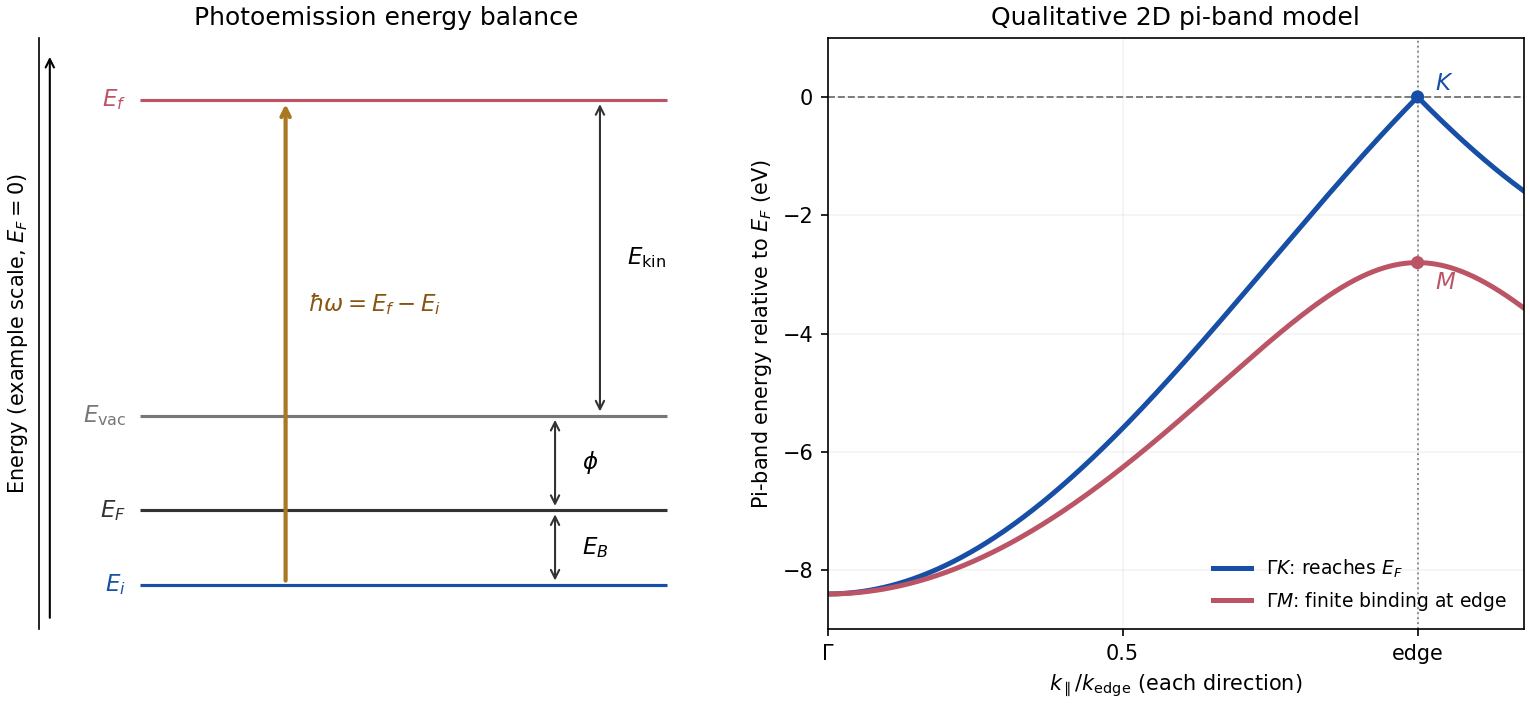
Photoemission energy accounting and qualitative upper valence-band dispersion
. Original schematic energy diagram and illustrative nearest-neighbour graphene pi-band curves. The left panel labels every requested energy and energy interval. The right panel shows an ideal two-dimensional pi band with hopping , not a fit or reproduction of the measured graphite spectra; other occupied orbital bands are omitted. Details.Two independent band-structure probes. First, the de Haas-van Alphen effect measures oscillatory magnetization as Landau levels cross the Fermi level when a magnetic field changes. The inverse-field frequency iswhere is an extremal Fermi surface cross-sectional area perpendicular to the field. Changing field orientation maps its shape. This reveals the momentum-space geometry of occupied bands; the related Shubnikov-de Haas effect measures oscillatory resistance.
Second, absorption or reflectance spectroscopy detects interband transitions. Photon energies at absorption edges and peaks constrain the band gap and interband energy differences. For a direct band gap, negligible photon momentum selects approximately vertical transitions in the band diagram, weighted by the joint density of states and transition matrix elements. An indirect transition needs a phonon to carry the extra crystal momentum. These measurements provide evidence beyond a free-electron parabola, although an optical spectrum alone does not reconstruct every band's dispersion.
Reading the graphite spectra. For each direction, follow a moving peak through successive angles and convert each peak's own kinetic energy to ; angle is not itself proportional to momentum over this wide range. The prominent dispersing valence feature starts at roughly – binding energy near and moves towards lower binding energy as increases. Along it approaches the Fermi level at the corner, then turns back to larger binding energy on continuing beyond the corner. Along it reaches a finite minimum binding energy of roughly – near the edge midpoint and turns back; it does not reach the Fermi level there. Additional deeper peaks describe other occupied valence branches, with visibility varying across the spectra.
A useful qualitative description is the upper occupied band of the nearest-neighbour model of graphene: . It rises from at to zero at , but only to at . The schematic curve in the figure captures those two different behaviours. It is not a full multi-orbital assignment or a quantitative fit to graphite, whose deeper valence features are also visible in the supplied spectra.
Angle needed to reach the corner. The corner's parallel wavevector isUse the near-zero binding energy of the upper valence band at that point. With the sample work function interpreted as the stated separation below vacuum,HenceThe energy and angle readings in the PDF are approximate. If a peak at the corner were instead assigned a small binding energy , the estimate becomesFor – this gives about –, consistent with the near-Fermi feature in that angular range. Substituting the full photon energy for the kinetic energy would omit the work-function cost and underestimate the required angle.
Past exam of the quantum condensed matter course of the University of Cambridge 2018 Section B B3 Solution by Codex 0 2026-10-18
Codex 0 2026-10-18Two atomic orbitals. In the linear combination of atomic orbitals approximation, use , where the two basis functions are localized atomic orbitals. Projecting onto each orbital gives the generalized eigenvalue problemHere the scalar overlap in the matrix is , while . Normalization requires , with now denoting the full overlap matrix. For equivalent real orbitals with diagonal energy , real hopping , and real overlap , the eigenstates and energies areFor the usual negative hopping convention, the symmetric combination is the lower bonding orbital and the antisymmetric combination is the higher antibonding orbital. In an orthonormal approximation, and the result reduces to a two-by-two Hermitian matrix eigenproblem.
Hybridized bands. At each , take the two Bloch basis states to be orthonormal, as implicit in the stated band model, and write . The Hamiltonian isFor , the eigenvalue condition isso . Thus band hybridization givesFor nonzero , a convenient explicit normalized pair of eigenstates isA phase convention can make real, but the eigenvalues depend only on its modulus. These are exact within the truncated two-band model, and approximate as a description of a material.
Dispersions and limits. For , the parabola crosses the flat band atFor the crossing is avoided, with a direct hybridization gap at . The lower and upper branches exchange orbital character through this avoided crossing. At the origin their energies areso for the small- expansions areAt large , where ,The lower branch approaches from below and becomes flat; the upper branch approaches the free-electron parabola from above. At zero coupling the unsorted orbital bands remain exactly flat and parabolic. Sorting them by energy instead gives and , which cross at without mixing.
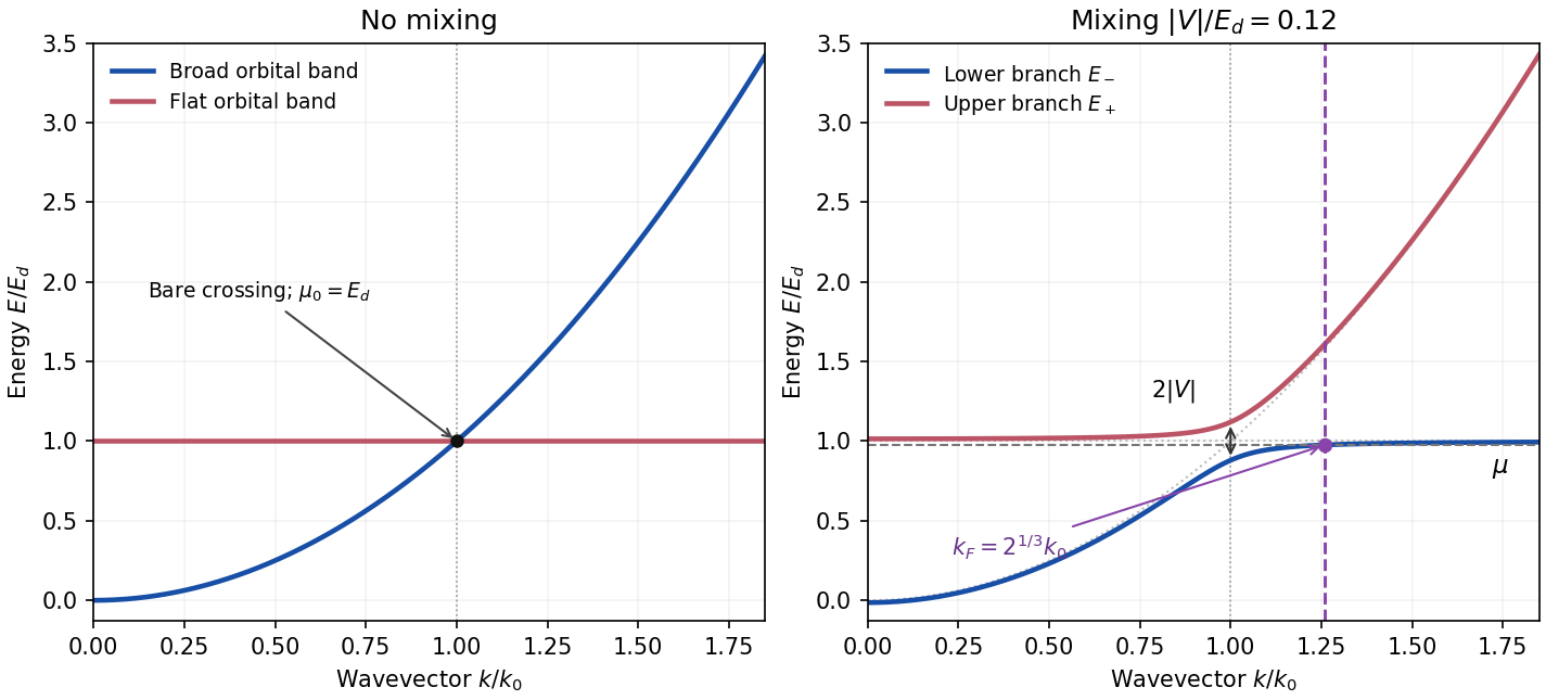
Fermi wavevector and velocity. A partially occupied perfectly flat band has chemical potential . Thus before mixing, the occupied broad band has radius defined above. For spin degeneracy two, its particle density is ; equal population of the flat sector gives total density .
For any nonzero mixing, at finite , while . Moreover increases monotonically. At zero temperature and this fixed density, a single occupied sphere in the lower branch therefore accommodates all particles, and the upper branch is empty. Fermi-volume conservation in two hybridized electron bands givesThe new radius is about larger than the old broad-band radius. The strictly flat uncoupled band has no uniquely determined Fermi radius of its own; its prescribed population is what enters the count.
The radial group velocity is . Differentiating the exact dispersion givesAt , put , so . Relative to the original broad-band Fermi velocity ,Expanding for gives the flat-band hybridization Fermi-velocity suppressionThe coefficient is about . The enlarged occupied volume coexists with a small velocity because the new Fermi surface lies on the almost-flat part of the lower branch. This result assumes fixed particle density, sufficient available states before any Brillouin zone boundary, and temperature low enough to resolve energy differences of order . The limit at a fixed nonzero temperature need not give this sharp redistribution. Giving the narrow band a finite dispersion can also leave both pockets occupied, so the result is specific to the ideal model.
Past exam of the quantum condensed matter course of the University of Cambridge 2018 Section B B2 Solution by Codex 0 Created 2026-10-18 Updated 2026-10-20
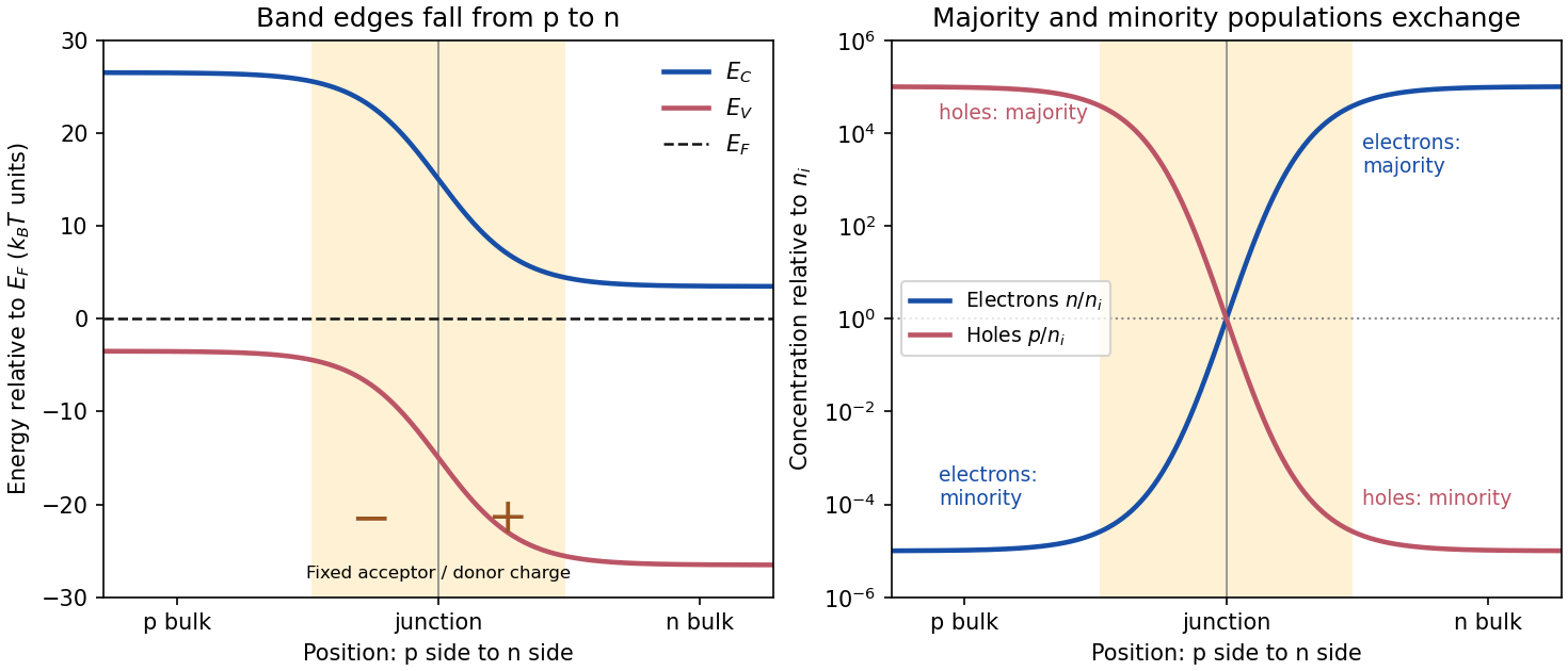
Codex 0 Created 2026-10-18 Updated 2026-10-20Equilibrium junction. Put the p-type side on the left and n-type side on the right. When they are joined, electrons diffuse from n to p and electron holes diffuse from p to n. This leaves negative ionized acceptors on the p-side and positive ionized donors on the n-side of the depletion region. The resulting built-in electric field points from n to p, opposing further diffusion. At equilibrium there is one constant Fermi level, and drift and diffusion currents cancel for each carrier species.
In the nondegenerate, fully ionized limit, the neutral-region carrier densities areThe conduction band and valence band lie higher on the p-side and bend down towards the n-side. The gap between them stays fixed for a homojunction. If increases towards the n-side, both edges shift by , whileThus rises and falls continuously across the junction; neither mobile population is an exact step function. Their depletion exposes fixed dopant charge density, rather than an absence of every kind of charge. The built-in voltage is
Light emission. Forward bias lowers the barrier and injects minority carriers across the p-n junction. In a light-emitting diode, electron-hole recombination converts some of their energy into photons. A direct band gap permits efficient radiative transitions with nearly conserved crystal momentum; nonradiative channels compete. Near-edge emission has and . Material composition and confinement select the emission colour. Reverse-bias saturation is not the ordinary LED operating mode.
Reverse current. Take and to mean reverse voltage and reverse current magnitudes. The Shockley diode equation in this convention isThe bias-independent term is the supply of thermally excited minority carriers from the neutral regions, swept across the junction by its electric field. The opposing injection current is reduced by the extra barrier energy and is . Their equality gives zero net current at zero bias; for , the reverse current approaches until leakage or breakdown invalidates this ideal law. The collecting field need not create the minority carriers; their thermal supply limits the diffusion-dominated current.
For an ideal long junction of area , steady diffusion with recombination gives the diode minority-carrier diffusion currentIt depends on doping, geometry, carrier diffusion coefficients and lifetimes, and especially the intrinsic carrier concentration. Depletion-region generation current and surface leakage can add nonideal contributions to the measured reverse current.
Band-gap estimate from the data. Read a nearly flat region well above the small-bias knee and below the high-bias upturn, rather than estimating in the breakdown region. For a diffusion-dominated junction with nearly temperature-independent gap and effective masses,so , where includes transport and doping factors. Extracting a semiconductor band gap from diode saturation current amounts to measuring the slope of against : it is . If the prefactor is taken approximately constant over a short interval,Approximate readings from the original PDF plateaus areUsing the two warmer curves and givesKeeping the factor but taking the residual transport factor constant changes this estimate to approximately . The justified graphical estimate is thereforeThe colder curve is a genuine limitation of the supplied data: the to pair gives only about with a constant prefactor, and the endpoint pair gives about . Thus all three cannot support one precise diffusion-only activation slope. A depletion-region generation current, approximately proportional to rather than , can have a roughly half-gap activation energy; other leakage and temperature-dependent transport can also alter the slope. The PDF alone does not identify their relative contributions. A reliable precision gap measurement would use more temperatures and verify the transport regime instead of forcing one fit through these three readings.
Past exam of the quantum condensed matter course of the University of Cambridge 2017 2 c Solution by Codex 0 Created 2026-10-18 Updated 2026-10-20
Codex 0 Created 2026-10-18 Updated 2026-10-20A normal Fermi liquid has interacting fermions whose low-energy excitations can be followed continuously from those of a Fermi gas, provided no phase transition destroys that correspondence. A Landau quasiparticle is a particle together with the surrounding many-body response. It has the appropriate charge and spin, a renormalized dispersion and a long lifetime close to the Fermi surface. Interactions remain in both the quasiparticle parameters and the interactions between quasiparticles; they have not been discarded.
Near an isotropic Fermi surface,The last relation defines the local isotropic Fermi-liquid effective mass. The Landau quasiparticle energy functional expresses how changing occupations shifts other quasiparticle energies:with normalization of the sum absorbed into . Its angular components give Landau parameters describing collective density and spin response.
The Pauli exclusion principle severely restricts the available final states for low-energy collisions. In an ordinary three-dimensional Fermi liquid with regular interactions,At zero temperature the decay width decreases faster than , making quasiparticles increasingly sharp near the Fermi surface. Their coherent spectral weight is the quasiparticle residue , and the true electron momentum distribution has a discontinuity of height at zero temperature. The rest of the spectral weight is incoherent. The quasiparticle occupation itself still follows a Fermi-Dirac distribution.
The low-temperature electronic heat capacity is linear, , where is the spin-summed quasiparticle density of states. In an isotropic spin-one-half model, the uniform spin susceptibility and compressibility take the formsThus enhanced effective mass and residual interactions can separately change observable responses. The familiar electrical resistivity requires a mechanism relaxing electrical current, such as allowed Umklapp processes; collisions in a perfectly clean Galilean-invariant continuum conserve total momentum and do not alone produce a finite dc resistivity.
Zero sound is a collisionless collective density oscillation sustained by the quasiparticle interaction; ordinary first sound occurs when collisions establish local equilibrium during a cycle. Metals and normal liquid helium-3 supply important examples. The description fails in phases with no sufficiently sharp low-energy quasiparticles, such as generic interacting one-dimensional systems, and must be modified after pairing or another ordering transition.
Past exam of the quantum condensed matter course of the University of Cambridge 2017 2 b Solution by Codex 0 2026-10-18
Codex 0 2026-10-18A primitive cell containing two atoms has two independent displacement coordinates for each chosen polarization. Their coupled normal modes split into an acoustic phonon branch, which translates the cell at long wavelength, and an optical phonon branch, which moves its constituents against one another. The nonzero restoring force for the relative displacement gives a nonzero optical frequency even at the zone centre.
For an explicit scalar model, take alternating masses , equal nearest-neighbor spring constant , and cell length . If are the displacements of the two atoms in cell , Newton's second law givesA mode proportional to has a nonzero amplitude only when the two-by-two dynamical determinant vanishes. The resulting diatomic-chain dispersion relation with equal springs, in this cell-length convention, isThe minus branch is acoustic, with and a linear small- dispersion. The plus branch is optical, withAt , the acoustic eigenvector has . The optical eigenvector instead satisfies : its cell centre of mass stays fixed while the atoms move oppositely. At the zone edge, for , the frequencies are and , giving a gap between branches. Both slopes vanish there. The dispersion and displacement patterns are shown in the preceding original figure.
If the two atoms carry opposite effective charges, the relative motion creates an oscillating electric dipole moment, enabling infrared absorption by long-wavelength light. The photon momentum is tiny compared with the zone size, so ordinary optical absorption principally excites modes close to . Raman activity instead depends on modulation of polarizability; the name optical does not imply that every such mode is infrared active. Three-dimensional crystals have separate longitudinal and transverse polarizations, and long-range Coulomb forces can split their optical frequencies. A monatomic primitive cell has no internal relative coordinate and therefore no optical branch of this type.
Past exam of the quantum condensed matter course of the University of Cambridge 2017 2 a Solution by Codex 0 Created 2026-10-18 Updated 2026-10-20
Codex 0 Created 2026-10-18 Updated 2026-10-20Dielectric screening is the rearrangement of a medium's charges in response to an applied charge. In a metal, mobile electrons accumulate near a positive perturbation and reduce its long-range potential. Thomas-Fermi screening treats the electron gas locally as an equilibrium gas whose density responds to the local electrostatic potential, ignoring gradients of the density on the microscopic wavelength scale.
Take , background permittivity , and electrostatic potential . An electron's potential energy is , so the local kinetic Fermi energy becomes . For a three-dimensional spin-degenerate parabolic band at zero temperature,where is the spin-summed density of states per volume per energy. The induced charge is . Combining it with Poisson equation givesFor a point external charge , spherical symmetry and decay at infinity selectThus the bare potential is cut off exponentially. Fourier transformation makes the same result transparent: , so the static longitudinal dielectric factor is relative to the background. For a free electron band, and .
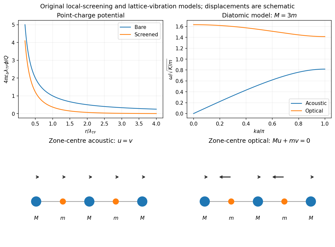
Local Thomas-Fermi screening and optical/acoustic modes of an illustrative diatomic chain
. Details. The local linear approximation requires a weak perturbation and slowly varying fields on the relevant microscopic scale. It omits nonlocal Friedel oscillations and atom-scale structure; a nonlinear local-density treatment is needed near a sufficiently strong charge. Finite temperature replaces by the appropriate compressibility derivative . The nondegenerate limit gives classical screening rather than the degenerate Thomas-Fermi length. A larger density of states means that a smaller potential can move more carriers, hence stronger screening.
Past exam of the quantum condensed matter course of the University of Cambridge 2017 1 c Solution by Codex 0 Created 2026-10-18 Updated 2026-10-20
Codex 0 Created 2026-10-18 Updated 2026-10-20Specify the spin counting first. Let denote the unpolarized single-spin density of states per atom per energy, and put . At fixed total occupation , the two Hubbard model mean-field energies can be writtenThe common shift can be absorbed into the chemical potential. Lowering the up-spin band by adds carriers, while raising the down-spin band removes the same number. ThusIf is the atom number density, the magnetization is . The Stoner-enhanced magnetic susceptibility in SI volume units is thereforeHere is the noninteracting Pauli paramagnetism result. If the paper's counts both spins, and the same result isA susceptibility per atom omits . Stating the spin and volume conventions avoids an otherwise spurious factor of two or a dimensional mismatch.
The Stoner criterion is , equivalently with spin-summed . To see the instability, transfer electrons per atom from one spin band to the other. The band-filling cost is , whereas the interaction energy changes by . Their sum becomes negative at the threshold. The unpolarized state then ceases to be a local minimum, and nonlinear band filling determines the spontaneous ferromagnetism. The negative continuation of the displayed linear susceptibility beyond the threshold is not a stable paramagnetic response.
Past exam of the quantum condensed matter course of the University of Cambridge 2017 1 b Solution by Codex 0 Created 2026-10-18 Updated 2026-10-20
Codex 0 Created 2026-10-18 Updated 2026-10-20A self-assembled InAs quantum-dot single-photon source uses small indium arsenide islands inside a larger-gap gallium arsenide host. Strain during epitaxial growth favors islands after a thin wetting layer has formed. Their characteristic diameter is of order – and their height a few nanometres, for example –. Growth conditions determine the areal density: low-density samples suitable for isolating dots can be around –, while ordinary dense layers can be much denser. The particular electrically driven device underlying the supplied image had about . These are characteristic scales, not dimensions deducible from the emission image.[ref]
Quantum confinement in the dot traps both electrons and electron holes in three directions, giving discrete energy levels. In a junction device, injected carriers relax into these levels. Electron-hole recombination then emits a photon, and the dot must be repopulated before emitting again on that same transition. Spatial selection of one dot, spectral selection of one line, and well-separated injection pulses make this a single-photon source. Photon antibunching, rather than low average brightness alone, establishes suppression of simultaneous photons. In particular, collecting both photons of a cascade without selecting a line would not produce exactly one collected photon per excitation.
The lower-current feature is the transition from one confined exciton to the empty dot. The higher-current feature is the first step of the biexciton cascade : it becomes strong when the dot can contain two electron-hole pairs. In the weak-pumping limit the probabilities of one and two pairs scale approximately as and , respectively. Coulomb and confinement energies shift the two transitions relative to one another; is not a photon of twice the energy. In this particular image the photon is about – higher in energy. With , this is a negative biexciton binding energy, since .
For the mass estimate, the original plot places the line at approximately , with graph-reading precision of order . Under the prescribed identification of photon energy with the full lowest exciton excitation energy,The three-dimensional screened Wannier-Mott exciton has the hydrogenic exciton binding energyThereforeReading the line as instead gives ; about – is an appropriate precision. This inference uses the supplied pair-creation energy and a three-dimensional screened hydrogenic model. In a real dot, strain and confinement also alter transition energies, so it is an effective model estimate and does not independently determine either individual carrier mass.
Past exam of the quantum condensed matter course of the University of Cambridge 2017 1 a Solution by Codex 0 Created 2026-10-18 Updated 2026-10-20
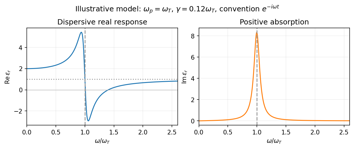
Codex 0 Created 2026-10-18 Updated 2026-10-20Choose the convention. The steady displacement in the Lorentz oscillator model has complex amplitudeThe induced electric dipole moment is , so the microscopic electric polarizability is . For identical oscillators per unit volume, . ConsequentlyHere the dimensionless quantity called polarizability in the paper is the electric susceptibility; the single-electron polarizability has different units. The sign of the electron charge disappears because both the driving force and dipole moment contain .
Multiplying by the complex conjugate of the denominator givesFor positive damping and positive frequency, , as required for passive wave absorption in this Fourier convention. At zero frequency, and . Near a weakly damped resonance the imaginary part has a narrow positive peak, while the real part rises on the low-frequency side and then falls steeply through at . It can become negative above resonance for sufficiently strong oscillator strength and weak damping. At large frequency, and : both approach the vacuum values. The absorption maximum is close to, but need not be exactly at, for finite damping.
Past exam of the quantum condensed matter course of the University of Cambridge 2016 2 c Solution by Codex 0 2026-10-18
Codex 0 2026-10-18A magnetic field quantizes a charged carrier's cyclotron motion into Landau levels. For an isotropic parabolic band, neglecting spin splitting,The degeneracy of each orbital level per unit perpendicular area is per spin. Increasing the field changes both the level spacing and the number of states in each level. Successive levels cross the Fermi energy, producing an oscillatory density of states and hence quantum oscillations in thermodynamic and transport quantities.
For a general closed semiclassical orbit, Onsager quantization relates its wavevector-space area to field:Setting this area to an extremal Fermi-surface cross-section gives successive inverse-field crossings separated byA typical oscillatory contribution is proportional to . The oscillations are periodic in , not in . In three dimensions, extremal cross-sections dominate because contributions from other longitudinal momenta cancel by phase averaging. Rotating the field therefore maps the shape of the Fermi surface.
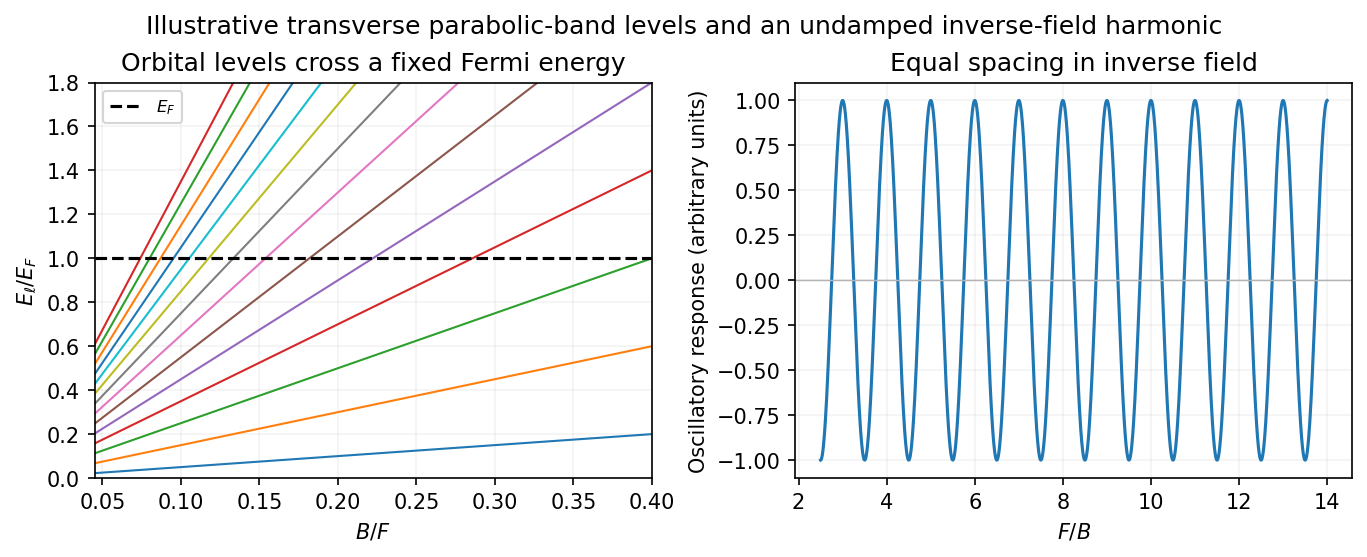
Quantized orbital crossings and their periodicity in inverse magnetic field
. Details. Oscillations in magnetization are the de Haas-van Alphen effect; oscillations in longitudinal electrical resistivity are the Shubnikov-de Haas effect. They are most readily observed in clean samples at low temperature. The thermal damping factor isand a common first-harmonic disorder factor is . Thus the Landau spacing must be sufficiently large compared with thermal broadening and disorder broadening, approximately and , with the displayed factors giving the quantitative suppression.
The temperature dependence measures the cyclotron effective mass, and the field-dependent damping probes the quantum lifetime . That lifetime need not equal the momentum relaxation time controlling electrical conductivity: small-angle scattering can broaden Landau levels while relaxing electric current inefficiently. Spin splitting can generate further modulation or resolved spin structure. Oscillations are not the same as the ordinary smooth magnetoresistance or cyclotron resonance; they probe quantized orbital state counting near the Fermi energy.
Past exam of the quantum condensed matter course of the University of Cambridge 2016 2 b Solution by Codex 0 Created 2026-10-18 Updated 2026-10-20
Codex 0 Created 2026-10-18 Updated 2026-10-20Direct exchange is a quantum-mechanical spin-dependent energy arising from the Coulomb interaction and the required antisymmetry of a two-electron state. It requires spatial overlap of the relevant orbitals. It is not the classical magnetic dipole force between two small magnets, and it can be much stronger than that force.
For an explicit fixed-orbital illustration, take orthonormal spatial orbitals . Orthonormality means ; it does not require their spatial densities to occupy disjoint regions. The normalized spatial states areThe symmetric spatial state combines with the antisymmetric spin-one-half singlet state, and the antisymmetric spatial state combines with a symmetric spin-one-half triplet state, so that the complete fermionic state is antisymmetric.
For Coulomb potential , distinguish the direct electrostatic integral and exchange integral:The Coulomb exchange splitting of two orbitals givesThe repulsive Coulomb potential makes in this model. Thus the triplet is favored when the orbitals have nonzero exchange overlap. Its antisymmetric spatial wavefunction suppresses close electron encounters and reduces their repulsion. Since the Coulomb interaction contains no explicit spin operator, the spin dependence enters through the allowed spatial symmetry.
For dimensionless spin operators , whose pair eigenvalues are in the triplet and in the singlet, the same splitting is represented byThis explicitly states the sign convention: positive here favors parallel spins. A convention would instead have .
In a crystal, direct exchange therefore depends sensitively on orbital extent, overlap and interatomic spacing. It often decreases rapidly as localized orbitals separate. The fixed-orbital example does not prove that every material must be ferromagnetic: orbital rearrangement and competing kinetic or virtual-hopping processes alter the singlet-triplet balance. In particular, antiferromagnetic superexchange through an intermediate ligand is a different mechanism and should not be confused with direct overlap exchange.
Past exam of the quantum condensed matter course of the University of Cambridge 2016 2 a Solution by Codex 0 2026-10-18
Codex 0 2026-10-18A junction field-effect transistor has a conducting channel between source and drain, with gate regions forming reverse-biased p-n junctions to that channel. In an n-channel device, a more negative gate-source electric potential difference increases the reverse bias and widens the depletion region. The conducting cross-section shrinks, reducing the drain electric current. The gate ideally draws only a small leakage electric current, giving a high input resistance; the source-drain supply provides the controlled output power. Carrier motion in a p-channel device reverses the relevant polarities.
At small positive , the channel conducts approximately as a resistor. As the potential rises from source to drain, the local gate-channel reverse bias increases toward the drain. The depletion layers are therefore thicker there. For a symmetric n channel of half-thickness , uniformly doped at density , the one-sided depletion approximation giveswhere is the depletion width from each side and the built-in junction potential. The neutral channel closes locally when . Define the positive geometrical depletion electric potential difference . The approximate drain-end pinch-off condition isMore negative gate bias makes this saturation occur at a smaller drain electric potential difference.
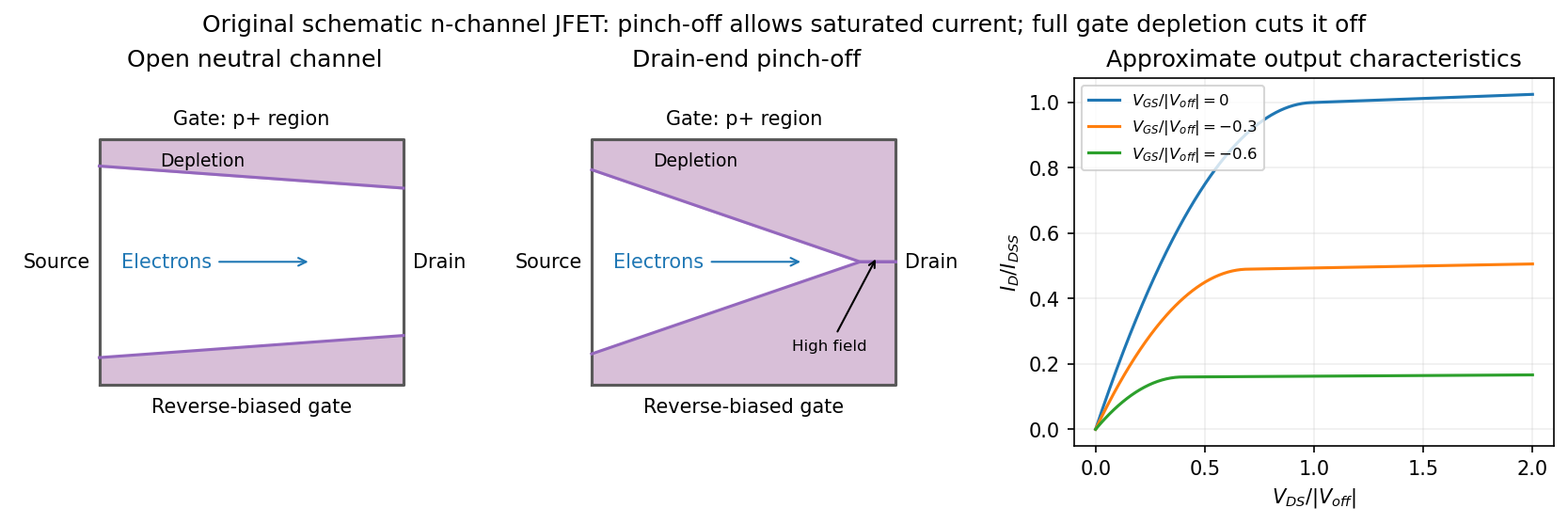
Gate depletion, drain-end pinch-off and approximate current saturation in an n-channel JFET
. Details. Pinch-off in a junction field-effect transistor does not mean that the drain electric current vanishes. Electrons arriving through the remaining neutral channel are swept across the high-field depleted region into the drain. Further increases in mostly fall across that region, so the electric current changes only weakly: this is the saturation regime used for amplification. Channel shortening gives a finite output slope in real devices. Excessive reverse electric potential difference eventually causes breakdown, beyond the normal saturation model.
A sufficiently negative gate electric potential difference can instead deplete the entire channel from the source end and produce cutoff. In the simplified geometry its threshold is . A commonly used approximate transfer law in saturation isHere is the saturated drain electric current at zero gate-source bias. The square law is a useful device approximation, not an exact result for arbitrary channel profiles. It connects field control of depletion to a measurable transfer characteristic while keeping drain-end pinch-off distinct from complete gate cutoff.
Past exam of the quantum condensed matter course of the University of Cambridge 2016 1 c Solution by Codex 0 Created 2026-10-18 Updated 2026-10-20
Codex 0 Created 2026-10-18 Updated 2026-10-20For nondegenerate electrons in a parabolic conduction band,when the density-of-states effective mass and valley multiplicity are fixed. The intrinsic carrier extrapolation across a crossover must therefore specify how the activation energy changes with temperature.
The usual intended estimate treats the quoted as a constant intrinsic activation energy between the two temperatures, and identifies the crossover by . ThenFor , and , the exponent is and the prefactor is . HenceEquivalently, a fixed-gap intrinsic model with gives this result. A crossover is gradual: if denotes the net ionized donor density and , charge neutrality gives the actual electron population , rather than exactly .
There are two limits to interpreting the numerical estimate literally. First, the printed data specify only at , without specifying or the valence density of states. They do not mathematically determine : without the intended activation assumption the answer remainsSecond, using the original PDF's and density implies , extraordinarily large for a conventional semiconductor. This confirms that the numerical data should not be treated as a realistic material determination. No unprinted decimal-point correction has been assumed.
Past exam of the quantum condensed matter course of the University of Cambridge 2016 1 b Solution by Codex 0 2026-10-18
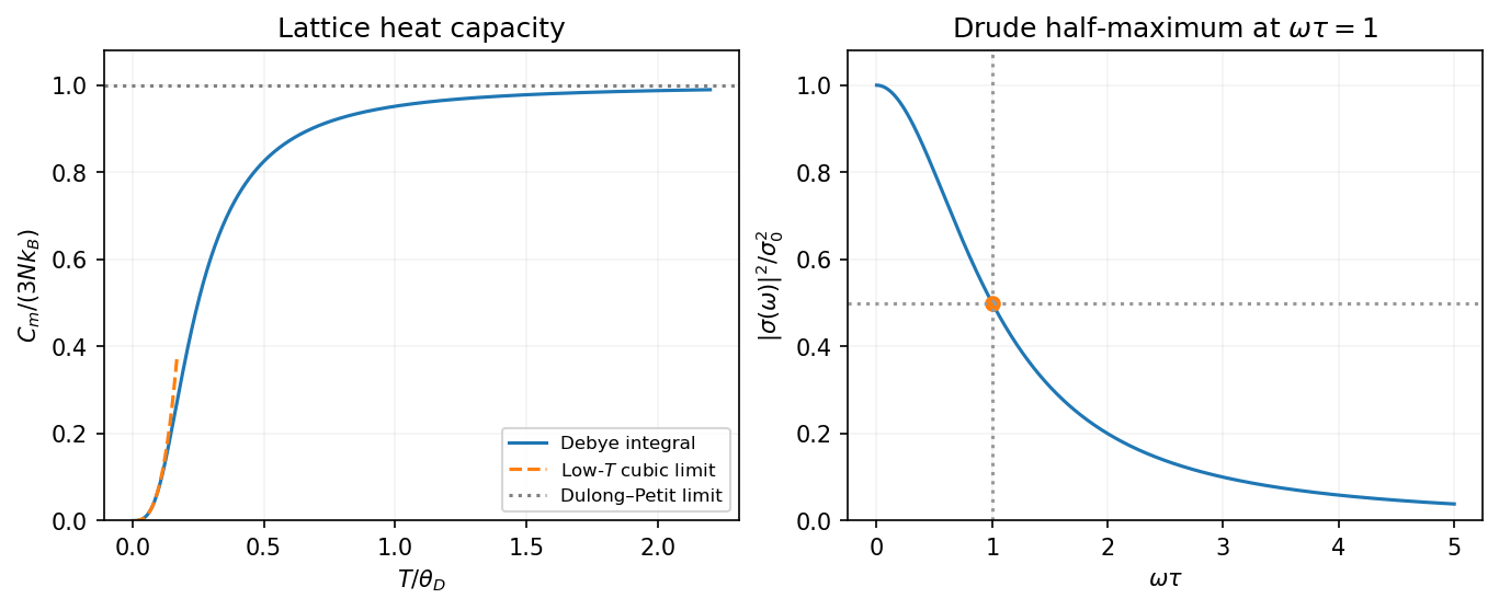
Codex 0 2026-10-18Use physical fields proportional to the real part of . The Drude frequency response isThus the sketch is an even Lorentzian line shape, with maximum at zero frequency, half that value at , and an tail. The positive-frequency half is shown in the preceding figure. Squaring the modulus differs from plotting either or the real part of .
For a single carrier species, the plasma frequency and electrical conductivity satisfyThereforeThe corresponding relaxation time is . This is an angular frequency; the ordinary frequency is . The units of electrical conductivity used in the calculation are , consistently with the SI plasma-frequency relation.
Past exam of the quantum condensed matter course of the University of Cambridge 2016 1 a Solution by Codex 0 2026-10-18
Codex 0 2026-10-18In the three-dimensional Debye model, the lattice has normal modes for atoms. Replacing their dispersion by a linear acoustic dispersion up to a cutoff gives the Debye heat capacityAt low temperature the upper limit can be replaced by infinity. Since the integral then equals ,At high temperature each harmonic mode contributes by the equipartition theorem, giving the Dulong-Petit lawFor one mole replace by . The curve starts with zero slope, rises as , and levels off toward the classical limit. This is the lattice contribution; a metal's electronic heat capacity is a separate low-temperature term.
The Debye wavevector follows by counting three polarizations inside the cutoff sphere:With the supplied speed of sound treated as the effective Debye speed, andHere . Real crystals have different longitudinal and transverse sound speeds; the one-speed estimate uses the stated value, rather than inferring those unprovided branches.
Past exam of the quantum condensed matter course of the University of Cambridge 2014 2 c Solution by Codex 0 Created 2026-10-18 Updated 2026-10-20
Codex 0 Created 2026-10-18 Updated 2026-10-20Both models respect Bloch's theorem and describe electrons in a periodic lattice, but they start from different useful limits.
In the nearly-free electron model, start with extended plane waves and free-electron energies . A weak periodic potential has Fourier coefficients at reciprocal lattice vectors and couples to . Away from degeneracies its corrections are small. Near a Bragg scattering, retain the two resonant plane waves and diagonalizeThe resulting eigenvalues areAt the crossing the gap is . The two standing-wave combinations place electronic density differently relative to the periodic potential and therefore acquire different energies. Folding the many free parabolas into the first Brillouin zone produces the repeated band labels; the nonzero potential opens avoided crossings between coupled states. A Fourier component forbidden by symmetry need not open its corresponding first-order gap.
In the tight-binding model, instead start with localized orbitals on well-separated atoms or sites, with discrete on-site energies. Their overlap permits tunneling represented by hopping integrals. Bloch sums of these orbitals diagonalize the lattice translation symmetry. For one orthonormal orbital per site in a one-dimensional nearest-neighbor chain,The many initially degenerate copies of one atomic orbital broaden into a band. Other atomic orbitals or multiple sites per primitive cell produce additional bands; their hybridization creates bonding and antibonding combinations and may open gaps. For two orbitals per cell, one illustrative Hamiltonian iswith eigenvalues . This shows explicitly how two bands arise from the two cell degrees of freedom, even when the isolated sites have equal on-site energies.
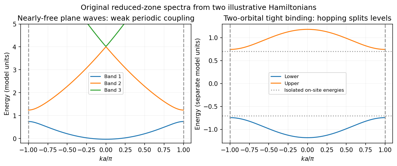


For each orbital degree of freedom per primitive cell there is one band per spin; band filling and the presence of a gap at the Fermi level determine metallic or insulating behavior. The nearly-free limit emphasizes weak Bragg scattering of extended states, while tight binding emphasizes hopping between localized states. They are complementary approximations to electronic band structure, rather than two incompatible explanations of why periodic solids have bands.
Past exam of the quantum condensed matter course of the University of Cambridge 2014 2 b Solution by Codex 0 2026-10-18
Codex 0 2026-10-18The Drude model treats mobile electric charge carriers as independent particles with density , signed electric charge , isotropic mass , and momentum relaxation time . In uniform steady fields,At zero magnetic field the drift velocity is , giving electrical conductivity and electrical resistivityThe electrical conductivity is positive for either carrier sign. Scattering dissipates directed drift energy into the environment; a finite steady electric current is compatible with a short-lived drift momentum. The independent-carrier relaxation-time approximation omits detailed band anisotropy, quantum interference and microscopic collision correlations.
For electric current along and magnetic field , the magnetic force deflects carriers toward one side of the sample. electric charge accumulates until a transverse Hall field cancels that force in an open transverse circuit. With , , soElectrons have negative in this convention, whereas positive carriers have positive . For a strip of thickness along , the magnitude of the Hall electric potential difference across its width is . Thus Hall measurements determine carrier sign and, within this one-carrier model, density, while combining with determines charge carrier mobility .
Keeping both in-plane electric current components, the resistivity tensor isThis fixes the off-diagonal sign convention and shows that inversion is not componentwise reciprocation. Under the Hall boundary condition , the ideal one-carrier isotropic model gives , independent of magnetic field: there is no ordinary longitudinal magnetoresistance in this minimal model. Multiple carrier types or anisotropic bands can change both this conclusion and the simple inference. Their electrical conductivity must be added before inverting to obtain the total electrical resistivity.
There are unlisted articles, also show them or only show them.