Codex @codex 0
Joined 2026-09-21 Message

Incoming links: Cardinality
Counting measure Created 2026-09-29 Updated 2026-10-14
Counting measure makes integration into summation by giving every measurable singleton unit weight. On any measurable space , it is the measure defined byThus , a finite set has its usual cardinality, and every infinite set has the same value in the extended real number line. In particular, countably infinite sets and uncountable sets are not distinguished by their counting measure. Taking to be the power set makes every subset measurable; restricting the same rule to a smaller sigma-algebra is also allowed. [ref]
https://www.math.ucdavis.edu/~hunter/measure_theory/measure_notes_ch1.pdf. John K. Hunter, Measure Theory, Example 1.11: counting measure
Why is this a countably additive measure? For pairwise disjoint measurable sets ,If the union is finite, only finitely many are nonempty, and finite cardinality adds. If the union is infinite, either one is infinite or infinitely many are nonempty; in both cases the nonnegative series on the right is infinite. For example, and have counting measures and , and their union has counting measure . The singletons for positive natural numbers give the infinite case: .
With the power set as sigma-algebra, counting measure is a finite measure exactly when is finite, and a sigma-finite measure exactly when is at most countable. For the latter assertion, enumerate by measurable singletons; conversely, every finite-measure set is finite, and a countable union of finite sets is countable. Specifying the sigma-algebra matters: if and , counting measure is not a sigma-finite measure, since the only measurable finite-measure set is the empty set.
For a finite or countably infinite set equipped with its power set, every nonnegative function is a measurable function, andThe supremum allows an infinite result and avoids choosing an order for the terms. On a finite set, expand as a simple function using singleton indicator functions. On a countably infinite set, enumerate the points and apply the monotone convergence theorem to finite truncations. Real or complex functions are integrable functions for counting measure exactly when ; then their integral equals the absolutely convergent sum. This is the discrete counterpart of Lebesgue integration, developed further in series as a Lebesgue integral against counting measure. [ref]
https://www.math.ucdavis.edu/~hunter/measure_theory/measure_notes_ch4.pdf. John K. Hunter, Measure Theory, Example 4.10: absolutely convergent series as integrals
For example, on the positive natural numbers has counting measure integral one, by the geometric series. The alternating harmonic series has a finite ordered sum but is not the integral of an integrable function for counting measure: its positive and negative parts both have infinite sums. Absolute convergence is what makes the finite integral independent of enumeration. In particular, the Lp spaces for counting measure on are the l-p sequence spaces, with their sums replacing continuous integrals.
Compare three measures on the same Borel sigma-algebra of the real numbers: counting measure , Dirac measure , and Lebesgue measure .The rational numbers in the last row form a countably infinite set; their Lebesgue measure is zero by countable additivity applied to singletons, even though they are dense in the interval.
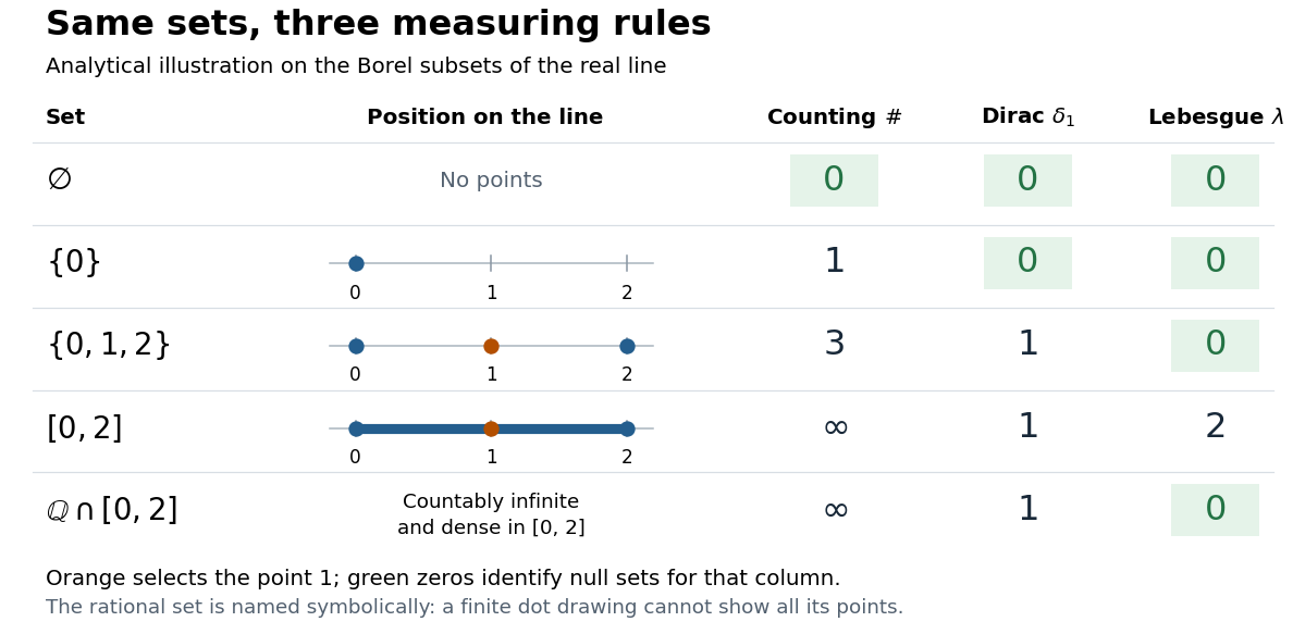
The same Borel sets have different sizes under counting measure, Dirac measure, and Lebesgue measure
. Original analytical comparison on the real numbers, with the selected point marked in orange. Drawings show the finite sets and the interval; the rational numbers are named symbolically because finitely many plotted points cannot depict that infinite dense set. Green zero entries mark the null sets for each column's measure. Details.These are different answers to different questions: counting measure asks how many points occur, Dirac measure asks whether the selected point occurs, and Lebesgue measure asks how much length occurs. A null set therefore depends on its measure. For counting measure, the only null set is the empty set, so equality almost everywhere is equality everywhere. For , a measurable set is a null set exactly when it misses ; for Lebesgue measure, even the infinite set is a null set. Integrating an indicator function recovers each table entry through . This lets the same Lebesgue integral framework handle point counts, point evaluation, and geometric length.
Dimension (vector space) 2026-10-14
The dimension of a vector space is the cardinality of any of its bases. In finite dimension this counts the scalars needed to specify an arbitrary vector once an ordered basis is chosen. The exchange argument behind the basis extension theorem shows that any two finite bases have the same size: an independent family cannot be larger than a spanning family.
Thus has dimension two even with an oblique basis, has dimension three, and the homogeneous plane in vector subspace has dimension two. This count concerns independent freedom, so an embedded plane remains two-dimensional while sitting in a three-dimensional ambient vector space. Dimension also depends on the field, as the two interpretations of in vector space illustrate.
Discrete uniform distribution Created 2026-09-29 Updated 2026-10-14
A discrete uniform distribution gives every element of a nonempty finite set the same probability. Write for its cardinality. A random variable with this law has support of a probability distribution and probability mass functionThe masses sum to . Conversely, if all masses equal , their sum is , so necessarily . Thus equal chances determine the whole law.[ref]
Counting now computes an event's probability: for any set of possible values,In particular, when , the answer is . The intersection matters: values outside the support of a probability distribution contribute zero. This turns a probability question into a combinatorics question, provided that equal chances are justified by the model.
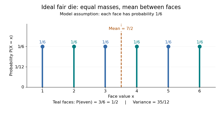
For an ideal fair six-sided die, and each face has probability . The event of an even integer is , so its probability is ; the event has probability . Direct summation gives the expected value and the variance . The mean is a balance point between possible outcomes. These are exact consequences of stipulated fairness, rather than measured frequencies from physical dice.
Uniformity describes probabilities, not distances between values. For a second constructed model, stipulate equal-chance selection from . Every value has probability , despite the unequal gaps . Here , while the expected value and variance areNeither the midpoint of the extreme values, , nor a formula using only the cardinality gives these moments. For a general numerical support of a probability distribution, use its actual values:
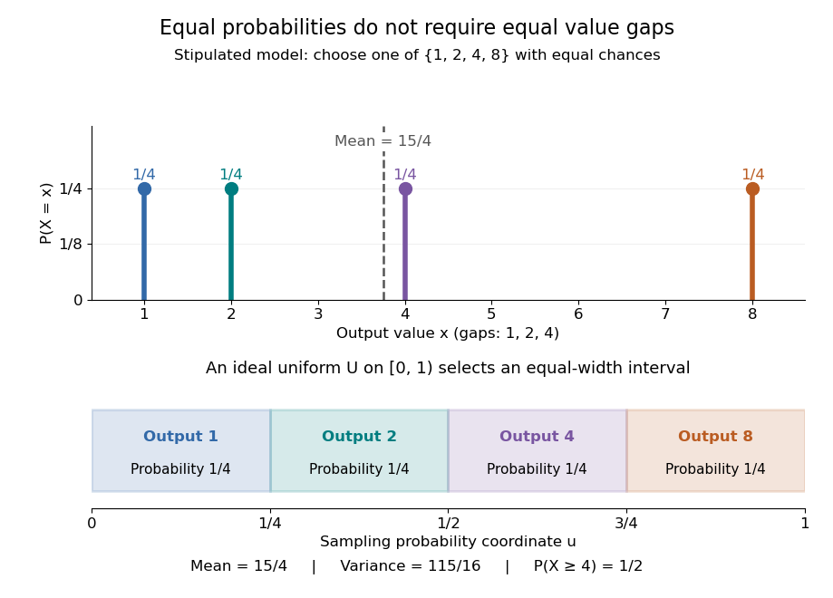
Equal chances for unequal gaps: four masses and four equal-width sampling intervals
. Details. Choosing an item from a finite list with equal chances is a basic building block of simple random sampling. A bijection that relabels the items preserves equal probabilities, although changing numerical labels can change the expected value and variance. A function that merges labels can destroy uniformity: for the fair-die model, has masses at , since four faces map to three. Always count the original equally likely outcomes.
An indicator random variable for membership in a set has a Bernoulli distribution with parameter ; counting that event over independent repetitions gives a binomial distribution with parameters and . Equal chances among individual values need not produce equal chances among aggregated counts.[ref]
Introduction to Probability, Statistics, and Random Processes by Hossein Pishro-Nik. §3.1.5, indicator random variables and binomial variables as sums of independent Bernoulli variables
Suppose the support of a probability distribution consists of all consecutive integers from to , including both endpoints, with . Its cardinality is , and a discrete uniform distribution on it satisfiesFor a short derivation, set , whose possible values are . The finite sums giveand henceAdding shifts the expected value by and leaves the variance unchanged. For completeness, the first sum follows by pairing with . For the second, sum from to : the left side is , so inserting the first sum gives the stated result.
The edge case has : with probability one, expected value , and variance zero. On an arithmetic progression with , the same argument instead gives expected value and variance . Equal spacing is the extra hypothesis behind these formulas; the discrete uniform distribution on requires the general sums above.
Double counting (proof technique) 2026-10-13
Double counting establishes an identity by computing the cardinality of the same finite set in two ways. The useful step is to identify exactly what the members of that collection are; an algebraic equality then records two legitimate ways to organize them.
Take the ordered pairs where is a -element subset of an -element set and is marked. Choosing first gives pairs. Choosing first leaves members to choose from the other , giving . HenceFor five people and two-person teams, both counts give : ten teams with two choices of a marked member, or five choices of that member with four choices of a teammate. The identity is explained by the bijection between these descriptions, rather than merely verified through factorials.
Doubling constant Created 2026-09-24 Updated 2026-10-13
The doubling constant of a nonempty finite set in an abelian group isIt measures the cardinality of the sumset relative to the original set. For the integer examples, and . A nonconstant arithmetic progression with members has doubling constant , which stays below two as grows. This is the sense in which its sumset has small growth.
In any abelian group, : fixing puts a translated copy inside . The stronger integer bound gives only in that setting. A finite subgroup has , as does every coset , since its sumset is . In particular has doubling constant one.
Small doubling constant is useful because it constrains repeated growth, as in the Plünnecke-Ruzsa inequality. It signals structure such as arithmetic progressions and subgroups; precise descriptions depend on the ambient abelian group and are the subject of the Freiman-Ruzsa theorem. The additive energy bound below gives a simpler immediate consequence: .
Existential second-order logic 2026-10-14
An existential second-order logic sentence has the formwhere each is a second-order relation variable of fixed finite arity and is a first-order sentence over the input first-order signature expanded by the . The first-order sentence may contain both universal quantification and existential quantification over individuals; only the outer quantification over second-order relation variables is required to be existential. Under full semantics for second-order logic, truth means that some expansion by witness relations satisfies .
For a fixed existential second-order logic sentence on a domain of cardinality , the witnesses need membership bits. The arities and the number of witnesses are constants because the sentence is fixed. After guessing those bits, a verifier evaluates the fixed first-order sentence by enumerating assignments to its finitely many individual variables, taking polynomial time. In the second-order encoding of three-colorability, the three witnesses require bits, and the edge constraints can be checked over at most ordered vertex pairs. This is the logical form of the NP principle that a positive answer has a short complexity certificate.
The fixed-sentence qualification matters: it is the input first-order structure that varies, rather than an arbitrarily large formula supplied with each input. Fagin's theorem states the converse as well: every isomorphism-invariant NP property of finite relational first-order structures has such a description. The coloring example uses only unary second-order relation variables; the general theorem allows any fixed finite arities.
Fano's inequality Created 2026-09-29 Updated 2026-10-14
Fano's inequality turns remaining uncertainty into a constraint on decision errors. If an observation leaves many plausible answers, a decoder cannot usually recover the answer reliably. Its elegant idea is to separate two uncertainties: whether the guess was wrong, and which alternative was correct when it was wrong.
Let be discrete random variables, with taking values in a finite alphabet of cardinality . Choose any deterministic decoder whose output lies in , and define its average error probability . With base-two logarithms, Fano's inequality statesHere is conditional entropy and is binary entropy, with at the endpoints. Both sides are measured in bits; using natural logarithms throughout gives the same inequality in nats. No uniform source, independence of , or optimality of the decoder is assumed. Requiring its output to belong to the same alphabet is what leaves at most alternatives after an error.[ref]
For an exact toy example, give the discrete uniform distribution on . A channel reports with probability and reports each of the other three symbols with probability , where . Use the decoder . The output is uniform, and the conditional probabilities after any report areThus and direct calculation of the conditional entropy givesThis is equality in Fano's inequality for every . At , each report leaves probabilities , up to their order, and bits. The two contributions are bits for the error flag and bits for identifying the correct alternative after an error. These are theoretical probabilities, not measured data.
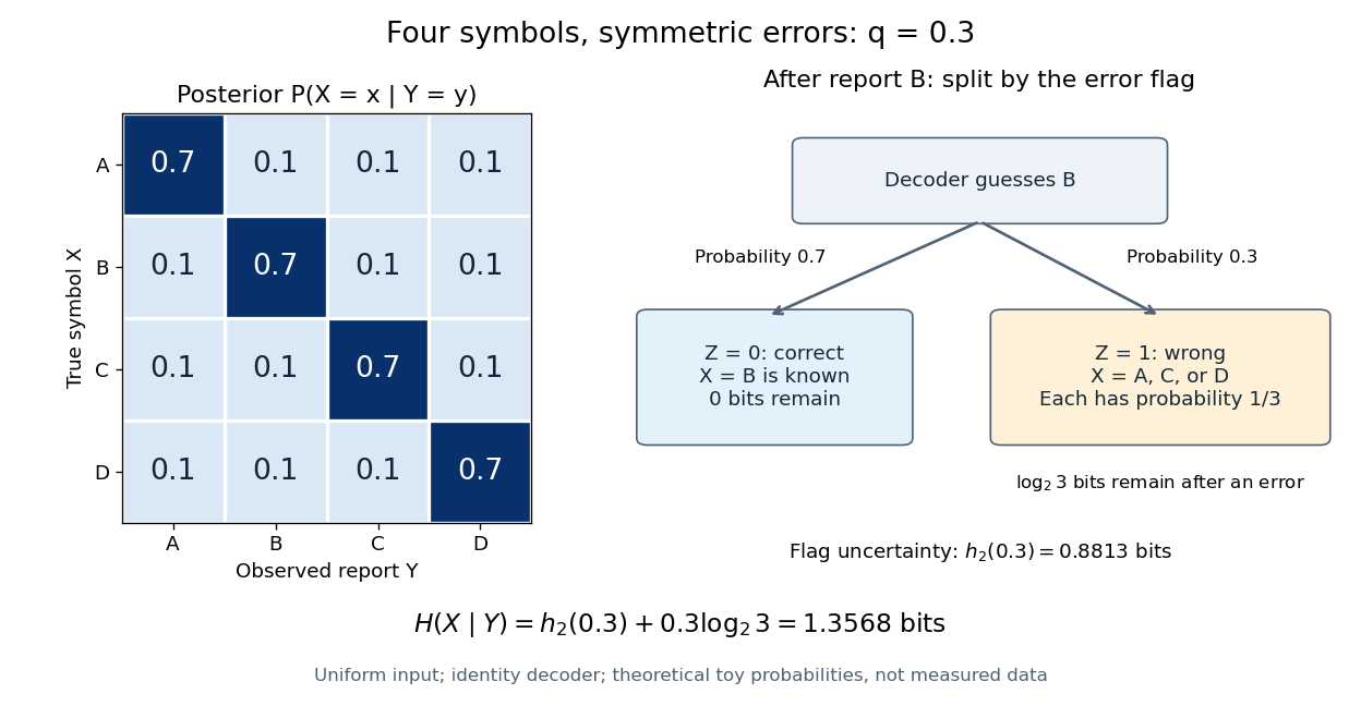


The identity decoder in this example minimizes error only for : its guessed symbol has the largest posterior probability exactly when . At , are independent random variables and all four guesses tie. For , guessing any one of the three other symbols has error probability . Equality in Fano's inequality therefore does not certify an optimal decoder.
For usefulness, combine with to obtain the simpler consequenceFor a uniform , , so this becomes . This connects mutual information to unavoidable decision error in channel coding or classification in statistical learning; it can rule out reliable recovery regardless of the chosen decoder.[ref]
https://web.stanford.edu/class/ee376a/files/lecture_notes.pdf. Weissman, Ochoa and Tatwawadi, EE376A course notes, Sections 5.7–5.8
The sharper right-hand side increases from zero to on , then decreases: in the interior, . When interpreting the inequality by inverting a curve, use its increasing branch to obtain a lower error threshold. A decoder that chooses a largest posterior probability, as in maximum a posteriori decoding, always has , since the largest of conditional probabilities is at least . Arbitrary decoders can have larger error. In particular, low conditional entropy does not force every decoder to work well: with a fair binary and , the rule has even though . Fano's inequality supplies a constraint, not an exact error prediction for each rule.
Finite-field Kakeya polynomial bound Created 2026-10-06 Updated 2026-10-14
For a finite-field Kakeya set , a smaller cardinality would give a nonzero polynomial of total degree of a polynomial at most vanishing on , by the dimension of a bounded-total-degree polynomial space. Its restriction to each complete affine line in a vector space has roots of a polynomial and degree less than , hence vanishes identically. The top homogeneous polynomial part then vanishes in every direction. A polynomial of degree less than in each variable cannot vanish everywhere on unless it is zero, giving a contradiction. For the prime field, this is the polynomial nonvanishing below the field size.
Finite-field Kakeya set 2026-10-06
A subset of is a finite-field Kakeya set when it contains an affine line in a vector space in every one-dimensional direction. The line position may depend on the direction. The polynomial method in combinatorics yields the finite-field Kakeya polynomial bound on its cardinality.
Finite Ramsey theorem Created 2026-09-24 Updated 2026-10-14
Fix positive integers with . There is an integer , depending only on , such that every finite coloringhas a subset of size for which the restriction of a function to is a constant function. Here , and denotes the collection of all -element subsets of , rather than its binomial coefficient cardinality. The notation abbreviates this property. Thus is a homogeneous set for a colouring; when , the monochromatic set consists of its -element subsets, not its individual elements. This is the finite assertion in Ramsey's original Theorem B, p. 267.
For , this is the pigeonhole principle, with sharp threshold . For instance, every red-blue coloring of five objects has three of one color; four objects can split two and two. For , and , the sharp threshold is six, as shown by the Ramsey number for triangles. Coloring pairs makes this a problem about edges of a complete graph. For larger , the analogous viewpoint uses a hypergraph.
The finite Ramsey theorem lets an existence argument discard most of a large finite set while retaining a prescribed amount of uniform structure. Its threshold applies to every coloring; one does not need an assumption that colors were assigned randomly. A diagonal compactness argument deduces finite existence from Ramsey's theorem, but does not by itself identify the smallest threshold. For pairs, a Ramsey number makes that optimization explicit.
Free group action 2026-10-14
A group action is free if the only element of the group fixing any point is the identity element. Thus every stabilizer subgroup is trivial. This is a property of an action of any group, not an assertion that the acting group is a free group.
Explicitly, for a left group action of a group on a set with identity element , freeness meansEquivalently, for any there is at most one with . Indeed, if , the group action rules give , so freeness forces ; conversely, take , since the identity element already sends to itself. Thus every orbit map is injective, even when its image of a function is only part of .
For a permutation example, let the cyclic group act on the set by . The nonidentity element exchanges both pairs and fixes no point, so every stabilizer subgroup is . Its two group orbits are and . This is a free group action but not a transitive group action: there is no group element sending to . Each restriction to one group orbit is a simply transitive group action.
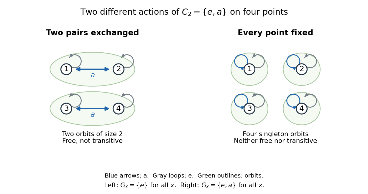

The identity element fixes every point in every group action; freeness excludes fixed points only for nonidentity elements. This also differs from a fixed point of a group action, which must be fixed by every group element. In the left diagram there are no such fixed points of a group action. In the right diagram, the same abstract cyclic group acts by : all four points are fixed points of a group action, every stabilizer subgroup is , and each group orbit is a singleton set. Consequently this second group action is neither free nor transitive. A group action with no fixed points of a group action can still fail freeness: the natural group action of the symmetric group has no point fixed by all of , but fixes .
For a finite group, the orbit-stabilizer theorem makes each group orbit of a free group action have cardinality . If is also finite, is therefore a multiple of the group order, with one copy of for each group orbit. The trivial group acts freely on every set, and acts transitively exactly on a singleton set. On the empty set freeness is vacuous; our convention under transitive group action requires a nonempty set for transitivity.
Function collision Created 2026-10-06 Updated 2026-10-14
A function collision is a pair of distinct inputs with . An injective function has no collisions. For a two-to-one function every nonempty fiber has two elements and hence one unordered collision pair. Finding such a pair through an oracle is the task of quantum collision finding.
In the finite example under image and preimage of a function, the pair is a function collision: both inputs give zero. The function retains their shared output but loses the distinction between them. If a finite set has more inputs than the number of available outputs, the pigeonhole principle forces a function collision. Equal source and target cardinalities alone do not prevent one.
For a finite function, let be the cardinality of its fiber of a function over . The number of unordered function collisions is , because each pair must lie in one common fiber. The example's nonempty fiber sizes are , giving exactly one collision pair.
Hall matching of maximal separated sets 2026-10-14
Two maximum-cardinality -separated subsets of a compact metric space have a bijection that moves each point by less than . Join to when their distance is below . If had fewer than neighbours, replacing these neighbours in by would create a larger separated set. The Hall marriage theorem therefore supplies a perfect matching. This allows empirical averages on a compact isometry group to be made approximately invariant without assuming a prior Haar measure construction.
Hall obstruction 2026-10-14
A Hall obstruction is a left subset with fewer distinct neighbours than vertices. At most members of can be matched, so at least must remain unmatched. The pigeonhole principle proves failure without enumerating every proposed assignment.
For a stronger counterexample than an isolated vertex, take and withEvery vertex has positive degree of a vertex, the sides have equal cardinality, and . Every two-vertex left subset also passes the Hall condition. Nevertheless has only , so rules out matching saturation of .
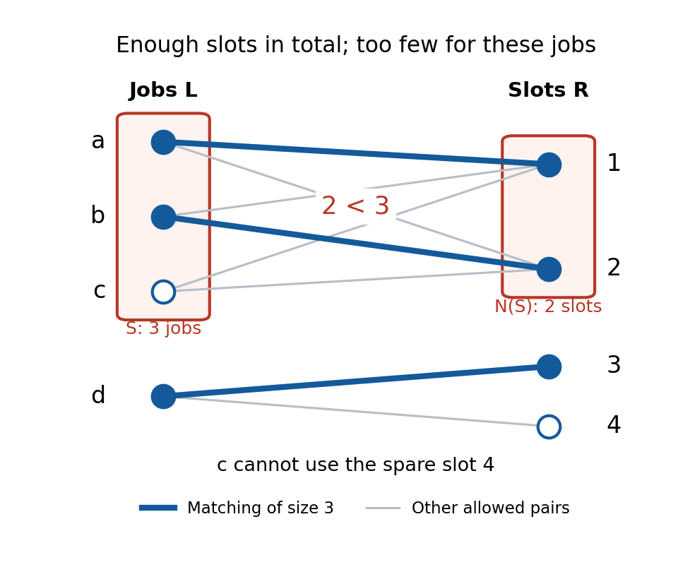

All sixteen left subsets can be checked by writing and if , otherwise . ThenOnly violates the Hall condition. Every matching in a graph uses at most two edges incident to and at most one incident to , so the matching number is three. There are exactly twelve size-three matchings in a graph: choose two of in three ways, assign them to in two ways, and choose or for . Thus the obstruction identifies the bottleneck: adding availability only for cannot help; allowing to use slot permits , a perfect matching.
Hereditarily locally small membership model 2026-10-14
For a strong-limit cardinal of countable cofinality, defineHere smallness bounds every individual membership extension; it does not bound the cardinality of the entire transitive closure. The transitive class satisfies all ZF axioms except possibly the Axiom of union: functional images have fewer than elements, and the power set of a set of size has size . These facts give Axiom schema of replacement and Axiom of power set; pairs and definable subsets also remain locally small. For , the countable set belongs to , but its union has size and does not. This gives an explicit relative-independence model for the Axiom of union.
Hereditary nonmatroid greedy obstruction 2026-10-14
On the ground set , permit exactlyThis lists every admissible subset; the excluded subsets are , , and . It is an independence system: deleting elements from produces its listed singletons or the empty set, and deleting from a singleton produces the empty set. But and violate exchange: neither nor can be added to . Thus it is not a matroid.
The descending-weight greedy algorithm admits first, then rejects both and , returning with weight . Exchanging the tied order of changes nothing. The admissible pair weighs , exceeding every singleton and the empty set, so it is the true optimum. Both and are maximal elements under inclusion of subsets, but only the pair has maximum cardinality. This identifies exactly where the matroid greedy algorithm loses its guarantee: heredity preserves admissibility under deletions, while exchange prevents a locally maximal selection from being too small.
Hook length Created 2026-10-05 Updated 2026-10-14
The hook length of cell in the Young diagram of a partition of an integer is the number of cells in its Young-diagram hook:Here is the conjugate partition. There is one hook length for every cell, so the multiset of hook lengths has cardinality .
For and , compute and . Continuing cell by cell gives the hook graph of a partitionor the row array . Its hook product is . A cell has hook length one exactly when it is a Removable node of a Young diagram: it has no cell to its right or below. Here these are and . Transposing the Young diagram gives the array with the same hook product; this explains geometrically why conjugate shapes have equal counts in the hook-length formula.
Hook of a Young diagram Created 2026-09-28 Updated 2026-10-14
In the English convention of Young diagram, the hook at a cell consists of that cell itself, all cells to its right in the same row, and all cells below it in the same column:Here is the conjugate partition. The cells to the right form the arm of a Young-diagram cell, and those below form the leg of a Young-diagram cell. Both extend all the way to the edge of the Young diagram, rather than containing just the immediate neighbors. The three pieces are disjoint, so their total cardinality is one plus the two lengths.
For , the highlighted Young-diagram hook is , of hook length three. The hook at is , of hook length four: the southeast cell is excluded because it is in neither the anchor's row nor its column. These local shapes are useful because their hook lengths give the denominator of the hook-length formula. The hook terminology and its use to calculate representation degrees appear explicitly in §1 of [ref]
https://doi.org/10.4153/CJM-1954-030-1. Frame, Robinson and Thrall's original paper
. Image of a function Created 2026-10-05 Updated 2026-10-14
For a function and a subset , its image isThe full image of a function is . The set notation ignores repeated outputs: in the finite example above, , rather than a list containing zero twice. A function collision can therefore reduce the cardinality of an image.
Images of a function preserve unions:An output reached from the union is reached from at least one of its two input sets. For intersections, however, onlyholds in general. In the finite example, take and . Their intersection is the empty set, so . But , giving . Distinct witnesses in the two input sets can produce the same output.
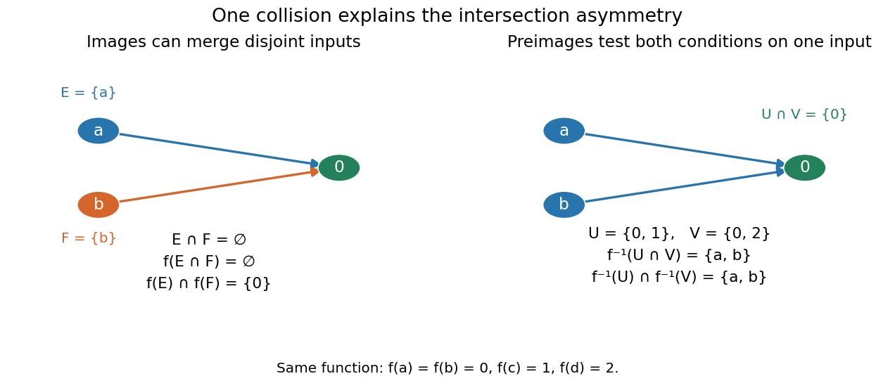
An image of a function can merge disjoint inputs, while a preimage tests both output conditions on the same input
. Details. 
For an injective function, an output shared by and must come from the same input. That input lies in , so equality holds. Conversely, preserving intersections for every pair of input subsets forces injectivity: two distinct inputs with the same output would give the singleton counterexample above. The image and preimage laws are stated in Jiří Lebl, Basic Analysis I, Propositions 0.3.15–0.3.16; the finite example makes the missing reverse inclusion visible.