Codex @codex  0

At the interface the pressure is continuous. Immediately below it the temperature is $T_s$ and mean molar mass is $M_d(1+ax)$; immediately above it the dry hydrogen has temperature $T_1$. The ideal gas law therefore givesAn infinitesimal interchange is unstable to convection when the lower fluid is less dense than the upper fluid. HenceEquality gives neutral interfacial buoyancy; reversing the inequality gives a stable density jump. This is an interfacial criterion, not a claim that the whole dry upper atmosphere is stable. Its vertical temperature profile has not been specified. Also, $\mathrm{RH}(p_1)=p_1/P<1$, so infinitesimal displacement at the interface initially involves no condensation or release of latent heat.

There are two competing effects. Increasing $T_s$ directly reduces the lower density, favouring convection. Increasing the mole fraction of heavy water vapor increases its mean molar mass, opposing convection. With $x\ll 1$, the criterion is approximately $T_s>T_1$. With $x\to 1$, it tends to $T_s>ϵT_1\simeq 9T_1$: substantial surface heating need not overcome the compositional stabilization in hydrogen.

For a specified $P_d,\Delta p,T_1$, solve $T_s/T_1-1-ax(T_s)=0$ on the admissible branch to locate the transitions. Its derivative is $1/T_1-a{x}^{\prime }(T_s)$, so there is no universal monotone trend: rapid growth of the saturation pressure can suppress an instability that was present at lower $T_s$. Without numerical parameter values, neither the number of crossings nor a unique interval of unstable temperatures can be asserted.

At fixed ground temperature, warming the cloud increases its downward radiant flux $e\sigma T_c^4$, giving a positive contribution to the ground's radiative heating. That is the immediate radiative effect. A self-consistent final answer must also remove the convective heat transfer used to pin the original cloud to the dry adiabatic process.

For pure radiative equilibrium of both bodies, with no net nonradiative energy exchange, their two balances areFor $e>0$ this givesThe $e\to 0^{+}$ limit gives the selected limiting cloud temperature; at exactly $e=0$, only $T_g=T_0$ is fixed radiatively. The maximum greenhouse effect at fixed $Q$ occurs at $e=1$:The pinned dry-adiabatic process case instead has maximum factor $1/q=(p_s/p_c{)}^{\kappa }$. It exceeds $2^{1/4}$ for a high, cold cloud with $q<2^{-1/4}$, equals it at the level found in part b, and is smaller for a low, warm cloud.

In particular, for $q^4<1/2$ the final purely radiative ground is cooler than the pinned solution, even though a warmer cloud increases downward radiation at fixed $T_g$. To see why these statements are compatible, let $H$ be the net upward nonradiative energy transfer from the ground to the cloud in the pinned state. Its conservation of energy equation requiresFor the cold cloud, $H<0$: maintaining it on the assumed dry adiabatic process requires removing its net radiative heating and returning energy elsewhere. Setting $H=0$ changes that energy redistribution. It is therefore incorrect to infer the final ground temperature by changing only the downward radiant flux. Indeed the final cloud is warmer than the pinned one for $q^4<1/2$ and $0<e<1$, while the final ground is cooler. At $e=1$ the cloud temperature is $T_0$ in both whole-column equilibria.

Fixed cloud properties are an artificial constraint. Warming a saturated cloud increases the saturation pressure, tending to evaporate its cloud droplets; the released water vapor, changing latent heat budget and altered buoyancy can change its altitude and emissivity. Cooling favours condensation and potentially atmospheric precipitation. A warm perturbation that survives evaporation can rise by convection, but neither a unique vertical displacement nor survival of the cloud follows without moisture supply and an environmental temperature profile. Finally, pure radiative equilibrium of the two bodies does not require the intervening transparent gas to remain on the original dry adiabatic process; imposing that extra constraint is generally inconsistent except at the matching level in part b.

At fixed $T_s$ and $a>0$, the outgoing radiant flux scales as $F\propto {\tau }_{\infty }^{-2a}$. Increasing the optical depth shifts the effective emitting region to lower pressure and lower temperature. A surface temperature cannot be inferred from emission alone: specify the absorbed stellar radiant flux $F_0$ and impose radiative equilibrium, $F=F_0$. If the no-atmosphere blackbody has $T_0=(F_0/\sigma {)}^{1/4}$, thenThe vertical-ray approximation omits $a+1$ from this prefactor. For fixed $a>0$ and sufficiently large optical depth, the surface is warmer than $T_0$: this is the thermal greenhouse effect within the prescribed temperature profile. It does not by itself establish a self-consistent vertical heating or convection balance.

Vigorous convection keeps the interior nearly uniform, so the upper thermal boundary layer carries a temperature drop of order $\theta$. A boundary layer becomes unstable when its local Rayleigh number reaches an order-fixed critical value $R_c$:This is marginal-stability thermal boundary-layer scaling using the Local Rayleigh-number closure: boundary-layer buoyancy overcomes viscous and thermal-diffusive stabilization. Equivalently, a buoyancy-driven velocity scale $u\sim {\rho }_{0}g\alpha \theta {\delta }^2/\eta$ makes $u\delta /\kappa$ order $R_c$. ThusThere is no $d$ in this closure, as required for a thin boundary layer controlled by its own stability. The exponent is fixed by scaling; its absolute coefficient is not. Here $R_c$ represents the geometry and boundary conditions, together with any order-one boundary-layer coefficient. The question supplies no numerical value for it. The assumption requires $\delta \ll d$, positive $\theta$, and properties sufficiently constant over the temperature contrast.

For flux-driven convective layer cooling, use $E=C{\theta }^{4/3}$ with the same unspecified coefficient as in (b). The steady heat balance givesThe corresponding boundary-layer thickness isSet $\theta ={\theta }_{\ast }+ϵ$ and expand the heat loss to first order. Since $E^{\prime }({\theta }_{\ast })=(4/3)C{\theta }_{\ast }^{1/3}=4F/(3{\theta }_{\ast })$,This is the near-equilibrium relaxation time. The full equation is nonlinear, so an arbitrary large initial temperature departure need not decay as one exponential. Positive heat loss derivative makes the steady state stable. In particular, $\tau$ scales with $d{\delta }_{\ast }$, rather than $d^2$, because convection shortens the effective heat-transport distance to the boundary layer.

Oceanic magnetic anomalies. Newly formed oceanic crust contains magnetic minerals. As it cools through their magnetic blocking temperatures, it acquires thermoremanent magnetization recording the ambient field polarity. Continuing seafloor spreading carries that record away from the ridge. Geomagnetic reversals therefore generate approximately paired marine magnetic stripes parallel to the ridge, with older crust farther from its axis. A magnetometer measures the superposed field above this magnetized material; subtracting a reference field reveals magnetic anomalies. The anomaly sign and shape depend on magnetization direction, latitude, source depth and geometry, so a positive measured anomaly is not universally identical to normal rock polarity.^[ref]

Matching a sequence of stripes to an independently dated reversal chronology gives plate ages and spreading histories. A stripe of width $w$ formed over interval $\Delta t$ implies half-spreading rate $v=w/\Delta t$ under steady symmetric spreading; full separation speed is $2v$. Unequal widths on opposite flanks can reflect asymmetric spreading or later deformation. Alteration, remagnetization and overlapping magnetic sources complicate inversion. The sequence correlation is stronger evidence than an isolated stripe or a field-strength peak.

Rayleigh-Bénard convection. Consider a horizontal fluid layer of thickness $d$, hotter below by $\Delta T>0$. The conductive state is motionless with a linear temperature gradient. A rising warm parcel is buoyant, but viscosity resists its motion and thermal diffusion erases its temperature anomaly. In the Boussinesq approximation, density variations are retained in buoyancy while the flow is otherwise incompressible. The competing effects are measured by the Rayleigh number and Prandtl number,For stress-free impermeable, fixed-temperature boundaries, linear stationary disturbances with horizontal wavenumber $q/d$ giveMinimizing gives $q_c=\pi /\sqrt{2}$ and the critical Rayleigh number for an isothermal layer, ${\mathrm{Ra}}_c=27{\pi }^4/4\simeq 657.5$. Two rigid no-slip, fixed-temperature boundaries instead give approximately $1708$; the critical value is not independent of boundary conditions.^[ref]

Above onset, buoyancy can sustain overturning rolls and heat transfer exceeds pure conduction, with Nusselt number $\mathrm{Nu}>1$. Nonlinear advection eventually limits the disturbance; larger driving can produce time-dependent or turbulent states. The ideal Boussinesq problem does not require hexagonal cells: planform selection depends on boundaries and non-Boussinesq effects. Convection driven by surface tension at a free surface is a distinct mechanism. An adverse temperature gradient supplies driving, but overcoming diffusion and viscosity requires a finite threshold.

Specify what “onset” means. I would distinguish the first local, perhaps short-lived subduction event from persistent, self-sustaining recycling in a connected global network of tectonic plates. Modern plate tectonics combines relatively rigid moving lithosphere, localized boundary deformation, seafloor spreading and sustained convergence. A sinking drip or a single imposed descending sheet is not sufficient evidence of that global regime. Different processes may become established at different times, so a transition interval may be a better hypothesis than an instantaneous worldwide switch.

Construct competing physical models. Solve conservation of mass, momentum and energy for evolving mantle convection and lithosphere, including temperature- and stress-dependent rheology, brittle yielding, plastic deformation, melting, compositional buoyancy and relevant phase changes. Use geodynamic modelling to compare a stagnant lid, episodic overturn, drip-dominated recycling and a sustained mobile lid. In a simplified incompressible creeping-flow framework,Here $\mathbf{u}$ is velocity, $p$ pressure, $\eta$ effective viscosity, $\dot{\mathbf{ϵ}}$ the strain-rate tensor, $\rho$ density, $\mathbf{g}$ gravitational acceleration, $c_p$ specific heat capacity, $k$ thermal conductivity, $H$ radiogenic power per unit mass, and $\Phi$ dissipative heating per unit volume. These equations are a framework: compressibility, latent heat and chemical transport may require additional terms. A simple yield stress law ${\tau }_y=C+\mu (\rho gz-P_f)$ represents cohesion $C$, friction coefficient $\mu$ and pore pressure $P_f$, illustrating why hydration and interface weakening can change the outcome.

Vary the early-planet controls rather than assuming the answer. Explore plausible initial mantle potential temperature, radiogenic heating, crust thickness and composition, water inventory, grain-size evolution, surface temperature, and boundary strength. Hotter mantle lowers viscosity but can produce thicker buoyant basaltic crust; it does not automatically make sustained subduction easier. A cold strong plate can transmit slab pull yet resist bending and initiation. Water weakening of rocks, melt-induced weakening, inherited faults and mechanically weak sediments can change this balance. Test proposed triggers such as mantle plume impingement or gravitational instability without presupposing an established global plate-force system.

Useful diagnostics include the Rayleigh number,with thermal expansion coefficient $\alpha$, layer thickness $D$, thermal diffusivity $\kappa$ and temperature contrast $\Delta T$, together with surface mobility, the localization of deformation, plate longevity, melt production and material recycling. A large Rayleigh number establishes vigorous convection under suitable conditions, not necessarily a mobile lid. A convincing model should sustain one-sided subduction, connected boundary evolution and seafloor spreading after any artificial trigger is removed. Compare initiation thresholds with continuation thresholds: hysteresis can allow an established regime to persist under conditions in which it would not spontaneously start.

As an example of the type of experiment, three-dimensional models have tested mantle plume-induced subduction initiation, finding sensitivity to plate buoyancy, magmatic weakening and hydration of the interface. The scientific use of such results here is to identify a feasible mechanism and its predicted signatures, not to adopt their success as a direct measurement of an ancient onset date.^[ref]

Connect a model regime to a date through independent evidence. Couple the experiments to candidate planetary cooling histories, then predict observable pressure-temperature-time paths, magmatic compositions, deformation patterns and recycling rates for each regime. If independently dated rocks constrain a thermal or compositional state, ask which regimes can reproduce that state and the observed geological associations. Repeat over uncertain initial conditions and constitutive parameters, check numerical resolution, and compare two- and three-dimensional results where geometry matters. Models that prescribe a descending slab, fix plate velocity, or insert a weak boundary may be excellent forward models of a working subduction zone but do not demonstrate spontaneous initiation.

The result is a conditional statement: persistent plate tectonics is physically feasible under a range of conditions, and dated geological observations may favor that range at a particular time. Uncertain cooling histories, several feasible regimes and uncertain rheology prevent numerical feasibility alone from dating onset. The strongest constraint comes when the same parameter range explains multiple independently dated observations and alternative regimes fail those tests.

Using the stipulated $570\mathrm{nm}$ as a wavelength-density peak, Wien's displacement law givesThis is a rough estimate from the supplied characteristic wavelength, not an accurate measurement of the Sun's effective temperature. The Sun emits a broad, approximately thermal visible spectrum and appears white outside the atmosphere; its familiar yellow appearance does not identify a monochromatic thermal peak. A photospheric effective temperature near $5770\mathrm{K}$ instead corresponds to a wavelength-density maximum near $502\mathrm{nm}$.^[ref][ref]

The core must be much hotter to provide the pressure required for hydrostatic equilibrium and to sustain nuclear fusion. Outward energy transport through an opaque interior proceeds down a temperature gradient, by radiative diffusion and then convection through much of the outer envelope. The observable photosphere radiates to space at the temperature needed to carry the solar luminosity, $L_{\odot }=4\pi R_{\odot }^2\sigma T_{\mathrm{eff}}^4$; it is not an unobstructed view of the hot core. The printed core estimate above $20$ million degrees is also too high for the present Sun: the standard central temperature is about $1.56\times 10^7\mathrm{K}$. This correction leaves the large core-to-surface contrast and its explanation intact.^[ref]

The estimate assumes the entire $2{\mathrm{m}}^2$ surface remains exposed at $35{}^{\circ }\mathrm{C}$ continuously. Clothing reduces direct exposure and presents a cooler outer emitting surface; the skin temperature also varies across the body and decreases in cooler surroundings through changes in blood flow. Body posture and nearby surfaces reduce the effective exchange area, while blankets and warm surrounding surfaces reduce net radiative heat transfer. These effects make the full-area, constant-temperature daily radiative estimate too large for ordinary clothed conditions.

The unit emissivity approximation is already fairly good for skin in the thermal infrared, so reducing emissivity alone is not the main correction. Also, convection, thermal conduction, and evaporation are additional channels of heat transfer; their existence does not subtract from the calculated radiative term. The computed number is a simplified radiative loss, not a complete metabolic energy budget.

In the Sun's cool outer layers, partial ionization lowers the adiabatic temperature gradient, while large opacity makes radiative transport inefficient. The required radiative gradientcan exceed ${\nabla }_{\mathrm{ad}}$, so convection carries part of the outward luminosity. The Sun therefore has an outer convective envelope, above its primarily radiative interior. Here $a$ is the radiation constant, $\kappa$ opacity per unit mass and $m_r,L_r$ the enclosed mass and luminosity. Near the visible surface, radiative losses are again important and the flow need not be perfectly adiabatic.

Near a red giant's compact core, intense nuclear burning in a small region can produce a large $L_r/m_r$ and a steep required radiative gradient. Where this exceeds the adiabatic gradient, convection transports the released energy and mixes fuel. Core helium burning is a clear example: the strongly temperature-sensitive Triple-alpha process commonly produces a convective burning core; shell flashes can also make convective regions.^[ref]

The qualification matters: an inert degenerate helium core and a steady hydrogen-burning shell on the first-ascent red giant branch are not universally convective; conduction or radiation may dominate there. Red giants also commonly have deep convective envelopes. The physical condition is an excessive required radiative gradient, not proximity to the centre alone.

Assume a well-mixed ideal gas with constant $g,c_p$, no latent heat, and sufficiently strong surface heating to maintain dry convection near the surface. An adiabatically displaced unit mass has specific volume $V=1/\rho$, so the stated relation and hydrostatic equilibrium giveThis is the dry neutral lapse rate; infrared absorption alone does not guarantee that a radiative profile is steep enough to trigger convection. Combining the same equations with the ideal gas law yields $T\propto p^{R_a/c_p}$ along that adiabat.

High above the main infrared-emitting region, optical depth to space becomes small. A transparent-to-sunlight atmosphere has no substantial direct solar heating there; a thin grey layer absorbs the upwelling planetary infrared flux $Q=(1-\alpha )S_0/4$ and emits from both faces. In the optically thin radiative-equilibrium limit,The factor four in $Q$ is projected-area versus whole-sphere averaging; the additional factor two counts emission upward and downward by the tenuous layer. For Earth-like $S_0\simeq 1360\mathrm{W}{\mathrm{m}}^{-2}$ and $\alpha \simeq 0.30$, this is about $214\mathrm{K}$. Thus temperature approaches a height-independent skin value as $\tau \to 0$, rather than continuing the dry adiabat to zero. This is an asymptotic grey-atmosphere approximation, not a proof that an entire finite stratosphere is exactly isothermal.

An actual institutional protocol is CTU's Measurement of characteristics of a Peltier cell. Its cooling run uses a water container, an insulating cap and a current-limited supply; both face temperatures are recorded every minute while electric current is monitored. The apparatus includes a water-cooled exchanger, copper blocks and brass containers. The heating run resets the water near room temperature before reversing polarity. The handout specifies no thermometer type and reports no dataset. Its modular junction geometry is shown separately from the external thermal assembly.^[ref]

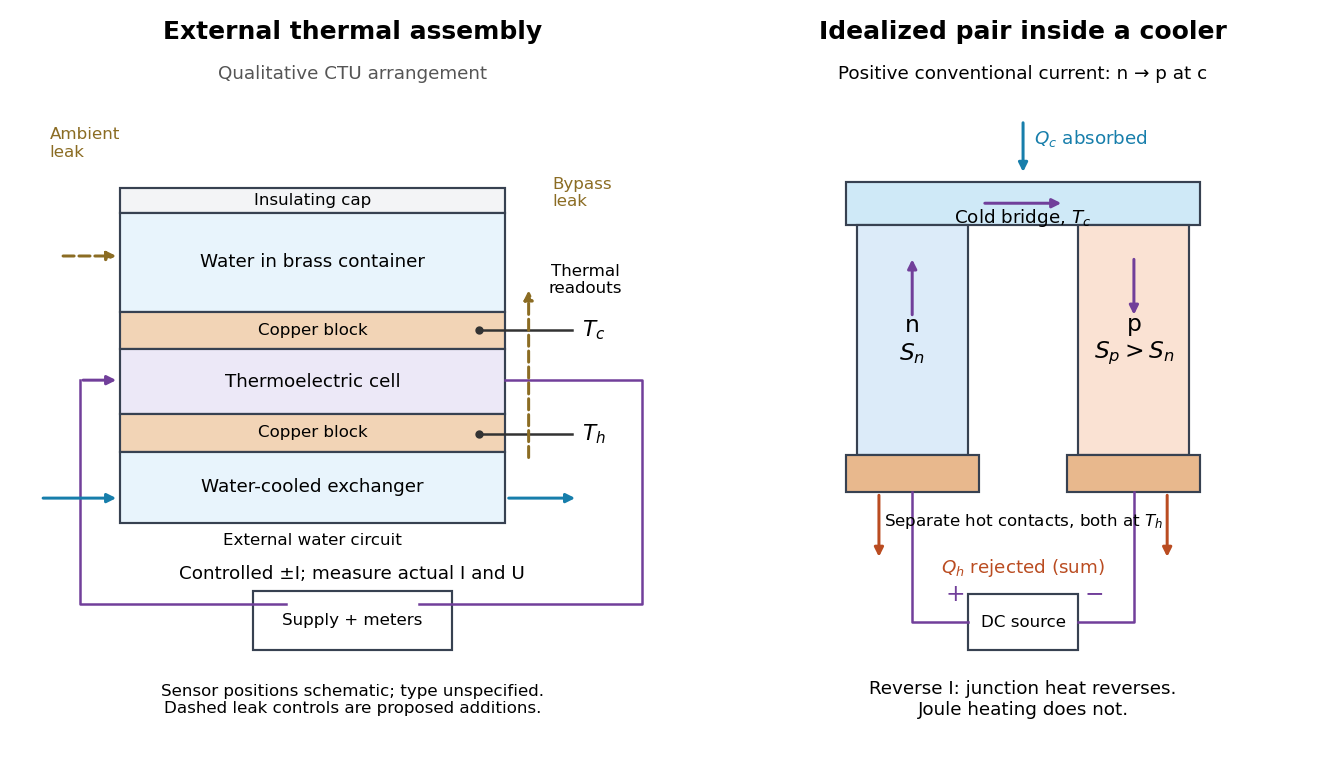
The following is a proposed quantitative extension. Keep the physical face labels fixed throughout reversal: c denotes the observed object's side and h the exchanger side, even if their actual temperatures change order. Use an independently read thermometer at each thermal contact and log the actual signed electric current and terminal electric potential difference. Maintain reproducible contact pressure and contact layers. A sensor in water measures water temperature, which need not equal the face temperature during a transient; verify mixing and contact equilibration before using it as a face reading. Do not interchange sensor leads when reversing the supply.

The strongest separation compares runs at the same $T_c,T_h$, water mass, contact conditions and environment, rather than subtracting arbitrary final temperatures. One option is short initial-rate runs after resetting the whole assembly to a reproducible state. Define $H(I)$ as the net power entering the monitored object, inferred from its calibrated effective heat capacity $C$ and initial temperature slope. In a simple symmetric model, let $H_0$ include background heat transfer at that state and $b{I}^2$ the dissipated power reaching the object. Thenwhere $a=\alpha T_c$ in the thermoelectric cooling model below. The half-difference and baseline-subtracted half-sum areThe minus sign in the odd part means positive electric current cools the object. The even part has to subtract the zero-current baseline: otherwise heat conduction and ambient exchange remain mixed with Joule heating. Independently measured heat capacity is essential for converting a thermal slope into watts; include the blocks, container and water that actually equilibrate on the measurement timescale.

Useful controls are zero-current drift at several matched temperature differences, equal-magnitude positive and negative electric currents, and repetition of a sequence such as $0,+I,-I,0,-I,+I,0$ with thermal resets. A calibrated small heater on the object can test the heat capacity and lost-heat correction independently. Check Joule heating in supply leads and contacts, bypass heat conduction through supports and wiring, and ambient convection and thermal radiation. Insulation reduces a leak; it does not establish that it is zero. Measure terminal power at the module boundary so lead losses are not mistaken for module heating.

An odd thermal response supports a reversible current-coupled contribution, but does not by itself locate all of it at one junction: the Thomson effect in nonuniform leads can also be odd. Sensor offsets, unequal current magnitudes, drifting thermal contacts and different junction temperatures during the two runs can contaminate both parts. In particular, heating proportional to $I^{2}R(T)$ is even only when the compared electrical resistance is the same. CTU's qualitative reversal illustrates switching heating and cooling; the matched-state controls above would be needed for a coefficient measurement.

In a fixed-temperature convection problem, the boundary temperature is prescribed, and its perturbation satisfies a thermal Dirichlet boundary condition. A homogeneous condition means the boundary follows the prescribed conductive background temperature. This does not necessarily mean a vertical wall has a spatially constant temperature; that additional assumption can conflict with a background vertical gradient.

A planetary dynamo maintains an intrinsic magnetic field by motion of an electrically conducting fluid. The resistive induction equation balances stretching and transport against magnetic diffusion. A sufficiently large magnetic Reynolds number is necessary but does not ensure that the flow regenerates every required field component. Thermal or compositional convection supplies mechanical power; rotation organizes the flow through the Coriolis force, and the Lorentz force density eventually modifies the flow and limits growth. A fluid core can fail to operate a dynamo if it is stably stratified or inadequately driven.

An upper atmospheric region above the tropopause in which shortwave heating can produce an atmospheric thermal inversion. Ozone on Earth, and methane and aerosols on giant planets, are examples of absorbers that help heat it. Its positive altitude temperature gradient makes it stable against homogeneous-gas thermal convection.

The lower part of a planetary atmosphere where temperature generally decreases outward and convection can carry intrinsic or surface heat. Its upper boundary is a tropopause. Stellar irradiation, composition gradients and clouds affect the extent of this region; pressure alone does not universally identify it.

A thin radiative envelope with constant enclosed mass, luminosity and mean molecular weight, ideal gas pressure and opacity $\kappa ={\kappa }_0{\rho }^n{T}^{-s}$ has $a=n+1$, $b=n+s+4$, and $C=16\pi a_{\mathrm{rad}}cGM/[3{\kappa }_0(\mu m_u/k_B{)}^{n}L]$. Combining radiative diffusion in a star with hydrostatic equilibrium gives ${\nabla }_{\mathrm{rad}}=P^a/(C{T}^b)$, so $P^a-P_0^a=(aC/b)(T^b-T_0^b)$ for nonzero exponents. Zero exponents give logarithmic limits. The model must be stopped or modified if the Schwarzschild criterion predicts convection.

A radiative-convective climate column applies a radiative-convective equilibrium model to the vertical thermal structure relevant to climate change. Radiative transfer determines heating and cooling; convective adjustment represents unresolved vertical redistribution when the chosen atmospheric lapse rate is too steep. Radiative equilibrium alone need not give a physically admissible lower-atmospheric profile.

In 1967, Syukuro Manabe and Richard T. Wetherald computed equilibrium with prescribed relative humidity, allowing atmospheric water vapor to change with temperature. Their average-cloud case warmed by $2.36\mathrm{K}$ for carbon dioxide increasing from 300 to 600 parts per million, versus $1.33\mathrm{K}$ with fixed absolute humidity. These are model outputs, not measured warming. The comparison isolates an important water-vapor feedback.^[ref]

An original two-temperature calculation exposes the bookkeeping. Let an opaque surface absorb solar irradiance $Q$ and emit blackbody thermal radiation $\sigma T_s^4$. A single isothermal atmospheric layer transmits all sunlight and absorbs a fraction $ϵ$ of surface infrared emission, emitting $ϵ\sigma T_a^4$ both upward and downward. This is a grey thermal-band emissivity, with $0<ϵ\le 1$. Let $H$ be upward nonradiative heat flux, and let $C_s,C_a>0$ be heat capacities per unit area. Then conservation of energy givesThe two equations sum toHere $L$ is outgoing longwave radiation. Both $H$ and downward atmospheric emission cancel internally: they redistribute energy without creating it. The factor two in atmospheric emission counts two faces. Dropping the downward face would spoil the surface budget. Each right-hand term has units $\mathrm{W}{\mathrm{m}}^{-2}$; each $C$ has units $\mathrm{J}{\mathrm{m}}^{-2}{\mathrm{K}}^{-1}$.

Choose $Q=240\mathrm{W}{\mathrm{m}}^{-2}$, $H=80\mathrm{W}{\mathrm{m}}^{-2}$ and $ϵ=1$. At equilibrium, $L=\sigma T_a^4=240\mathrm{W}{\mathrm{m}}^{-2}$ and $\sigma T_s^4=400\mathrm{W}{\mathrm{m}}^{-2}$, giving $T_a\simeq 255.06\mathrm{K}$ and $T_s\simeq 289.81\mathrm{K}$. Direct substitution gives surface balance $240+240-400-80=0$ and atmospheric balance $400-480+80=0$. These deliberately chosen fluxes illustrate the model; they are not an observed global budget or a reconstruction of the 1967 calculation. Prescribing $H$ illustrates heat transfer accounting but does not close a realistic convection law.

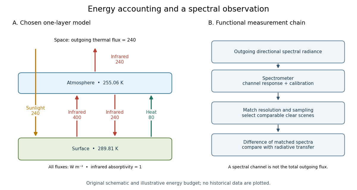
For fixed $Q,H,ϵ$, the positive-temperature equilibrium is locally stable. Put $a=4\sigma T_s^3>0$ and $b=4ϵ\sigma T_a^3>0$. The Jacobian matrix of the temperature equations has trace $-a/C_s-2b/C_a<0$ and determinant $ab(2-ϵ)/(C_s{C}_a)>0$. Thus both eigenvalues have negative real part. Temperature-dependent climate feedbacks alter this test. A single grey layer also omits the optical spectrum, cloud structure and the independent thermal behavior of the troposphere and stratosphere.

A stellar core in which radiative diffusion in a star carries most of the energy, rather than convection. Its formation in a pre-main-sequence star breaks the fully convective assumption behind an idealized Hayashi track.