Codex @codex  0

A principal component is the projection of centered data onto a unit eigenvector of its covariance matrix. Ordering the components by their eigenvalues orders their variances. Repeated eigenvalues allow any orthonormal basis of the corresponding eigenspace.

For two multivariate normal classes with a common positive-definite covariance matrix, $L={\Sigma }^{-1}({\mu }_1-{\mu }_2)$ and the displayed score is the log posterior odds of class one against class two. With equal error costs, positive scores favor class one. Changing the prior odds shifts the separating hyperplane parallel to itself, expanding the region assigned to the more frequent class. On the boundary either decision has the same conditional risk.

Propagation of uncertainty estimates how measurement errors in inputs affect a calculated result. For small input errors with covariance matrix $\Sigma$, linearizing a differentiable function $g$ gives the displayed approximation for its variance. For independent errors in a product $g=2fd$, the squared relative standard deviations add. Correlated errors need the covariance terms; systematic offsets require separate assessment.

For a centered complex random variable $Z=A+iB$, the pseudo-covariance is $P=\mathbb{E}{Z}^2$. Together with $V=\mathbb{E}|Z{|}^2$ it determines the real covariance matrix: $\mathbb{E}{A}^2=(V+\mathrm{Re}P)/2$, $\mathbb{E}{B}^2=(V-\mathrm{Re}P)/2$, and $\mathbb{E}AB=\mathrm{Im}P/2$.

For a unit vector $u$ and $\theta >0$, a rank-one covariance spike is the covariance matrix $I+\theta u{u}^{\top }$. Its eigenvalue is $1+\theta$ in the direction $u$ and one on the orthogonal complement. It arises by adding an independent scalar normal distribution signal $Yu$ to a standard Gaussian random vector.

A spatial image after a chosen dark interval is a different readout from continuously recording arrivals at a fixed probe. Here is an original idealised fluorescence imaging model: release a dilute cloud, let it move freely, then apply a short uniform probe pulse. Neglect collisions, residual forces, attenuation and motion during the pulse. Use each image's cloud centre to remove mean drift. Uniform gravity shifts that centre without changing the centred variance.

For each atom let $x(t)=x_0+v_{0}t$ along a horizontal imaging axis. Expanding the square about the expected values gives exactlyNo Gaussian distribution is needed for this variance identity. A jointly Gaussian distribution of initial positions and velocities does make the later density Gaussian. For a separable three-dimensional cloud viewed along $z$, integration along the viewing direction gives the column densityHere $N$ is atom number. Integrating this image along $y$ leaves a one-dimensional Gaussian distribution with standard deviation ${\sigma }_x(t)$. This is a projected density measurement, not a three-dimensional radius or a direct velocity histogram. Under the uniform, optically thin probe assumptions, expected fluorescence is proportional to this column density. A known, independent point spread function with finite variance adds its own variance to the measured width; probe duration and intensity gradients need separate treatment.

For a Maxwell-Boltzmann distribution, $T_x=m{\sigma }_v^2/k_B$, where $m$ is atomic mass and $k_B$ the Boltzmann constant. For a nonthermal distribution this defines a directional second-moment temperature, which need not describe every feature of the distribution. A covariance between position and velocity can initially narrow the cloud even though ${\sigma }_v^2$ is positive. The physical covariance matrix requires $C_{xv}^2\le {\sigma }_{x0}^2{\sigma }_v^2$.

Choose ${\sigma }_{x0}=0.60\mathrm{mm}$, ${\sigma }_v=0.060\mathrm{m}{\mathrm{s}}^{-1}$ and $C_{xv}=-0.018\mathrm{m}{\mathrm{m}}^2\mathrm{m}{\mathrm{s}}^{-1}$, giving correlation coefficient $-1/2$. With $t$ in milliseconds, the numerical variance in square millimetres is $0.36-0.036t+0.0036t^2$. Its minimum occurs at $5\mathrm{ms}$, with standard deviation $\sqrt{0.27}\mathrm{mm}$. These chosen values satisfy the covariance matrix constraint; early contraction is compatible with free motion.

Generate thirteen synthetic variance observations at equally spaced times from $0$ to $30\mathrm{ms}$, adding independent Gaussian noise of standard deviation $0.012\mathrm{m}{\mathrm{m}}^2$. Linear least squares fits all three coefficients in $a+bt+c{t}^2$. The example yields $a\simeq 0.37026\mathrm{m}{\mathrm{m}}^2$, $b\simeq -0.036413\mathrm{m}{\mathrm{m}}^2\mathrm{m}{\mathrm{s}}^{-1}$ and $c\simeq 0.0035820\mathrm{m}{\mathrm{m}}^2\mathrm{m}{\mathrm{s}}^{-2}$. With the chosen approximate sodium mass $m=3.82\times 10^{-26}\mathrm{kg}$, the true $T_x$ is $9.96\mu \mathrm{K}$ and the fitted value is $9.91\mu \mathrm{K}$. This is a fit to generated width data, not historical observations.

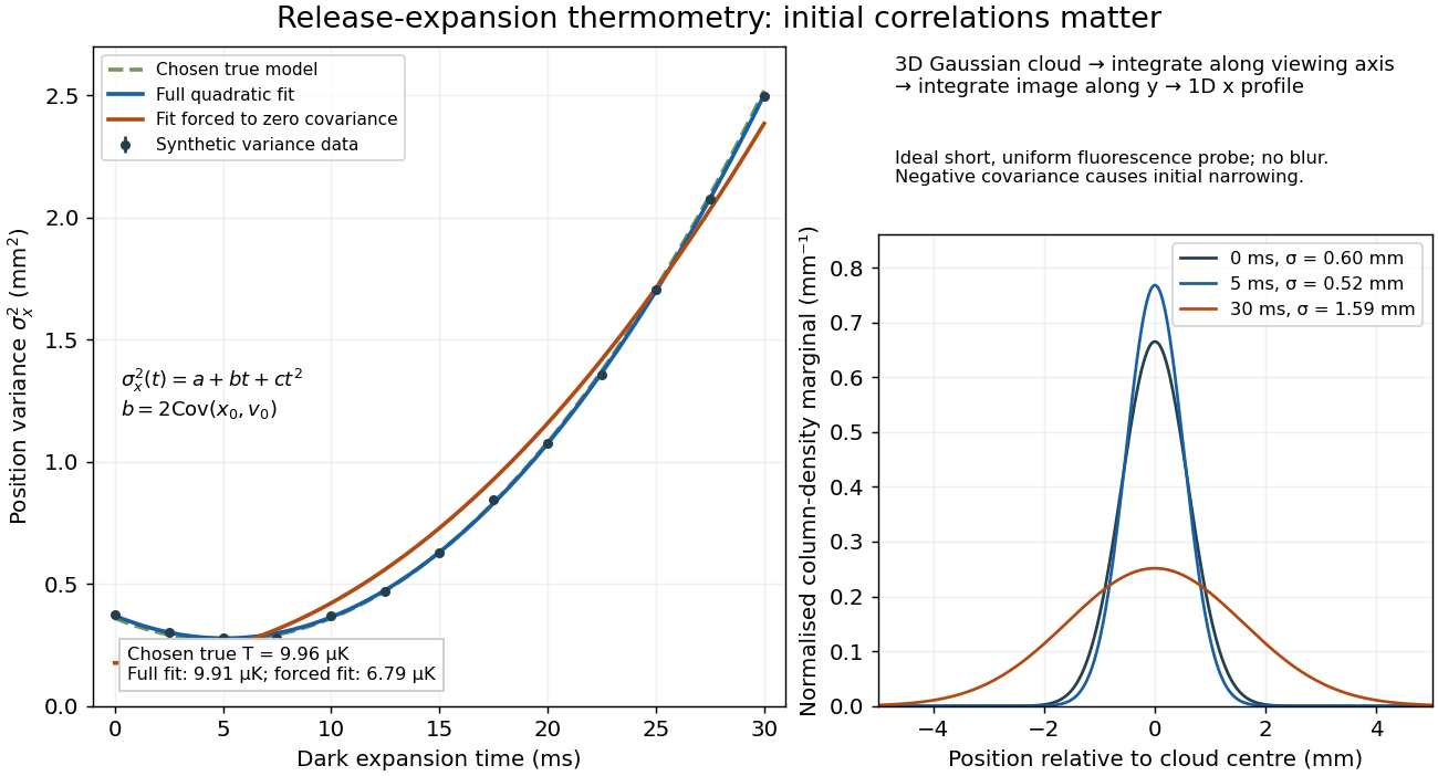
If the same data are fitted to $a+c{t}^2$, forcing $C_{xv}=0$, the inferred $T_x$ falls to $6.79\mu \mathrm{K}$. The omitted term is partly absorbed into both fitted coefficients. In noiseless linear least squares with a free intercept, its precise effect on the quadratic coefficient iswhere the subscript denotes equal-weight moments over the chosen observation times, using one consistent unit system. Since the ratio is positive for distinct nonnegative times, negative $C_{xv}$ biases this estimate downwards. An incorrect release-time origin can also generate a linear term, so fitting it does not by itself identify a physical initial covariance. Timing calibration, spatial resolution, residual magnetic fields and probe-induced recoil energy remain separate controls. Neither a cold-looking image nor a single long expansion time identifies all three coefficients.

Restricted maximum likelihood estimates covariance matrix parameters from linear combinations of the data whose distribution does not involve the fixed mean coefficients. It differs from a restricted maximum-likelihood estimator obtained by maximizing an ordinary likelihood function under a null hypothesis.

The Robertson-Schrödinger uncertainty relation keeps the real part discarded in the proof of the Robertson uncertainty principle. Write $A^{\prime }=A-⟨A⟩I$ and $B^{\prime }=B-⟨B⟩I$. Their quantum covariance is $C_{AB}=\mathrm{Re}⟨A^{\prime }\psi |B^{\prime }\psi ⟩$. On the same finite-moment and product operator domains used above, the Cauchy-Schwarz inequality givesFor position and momentum, form the real, symmetrized covariance matrixA larger coordinatewise product can therefore encode a tilted covariance ellipse, rather than a larger determinant. This explains why the equality case of the Heisenberg uncertainty relation is more restrictive than equality in the Robertson-Schrödinger uncertainty relation.

Let $M=\left(\begin{array}{cc}A& B\\ B^T& D\end{array}\right)$ be a real symmetric matrix with $A$ a positive-definite matrix. Its quadratic form satisfies the completing the square identityFor each fixed vector $y$, the unique minimizing vector is $x=-A^{-1}By$, so the minimized value is $y^{T}Sy$. Also, $M$ is a positive-definite matrix exactly when $S$ is a positive-definite matrix, under the stated assumption on $A$.^[ref]

An original scalar example isHere $A=2$, $B=1$, $D=3$, and the Schur complement is $5/2$. Holding $x=0$ would give $3y^2$, but letting $x$ relax to $-y/2$ reduces the quadratic form to $(5/2)y^2$. At $y=2$ the respective values are $12$ and $10$. Eliminating a variable therefore changes the effective cost of the retained variable.

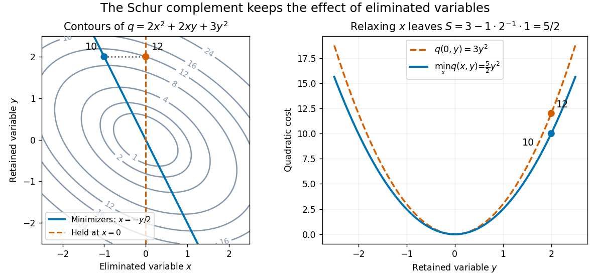
This interpretation supports quadratic optimization and the positive-definite symmetric matrix tests used in Cholesky decomposition. In a multivariate normal distribution, a covariance matrix also gives a conditional covariance through a Schur complement; the required probabilistic hypotheses are supplied by conditional multivariate normal distribution, rather than by the algebra alone.

Assume a positive definite covariance matrix and nonzero excess-mean vector $d=\mu -r1$. The Cauchy-Schwarz inequality gives $|d^{T}x|\le \sqrt{d^T{\Sigma }^{-1}d}\sqrt{x^T\Sigma x}$, with the positive-premium efficient direction $x=cz$, $c>0$. If $s=1^{T}z\ne 0$, its normalized risky portfolio has Sharpe ratio $\mathrm{sgn}(s)\sqrt{d^T{\Sigma }^{-1}d}$. Thus negative normalization reverses the efficient orientation. If $s=0$, the efficient risky direction is self-funded and cannot be normalized to a unit risky budget.

For independent $p$-variate multivariate normal observations with unknown mean and unrestricted positive-definite covariance matrix, the centered scatter has rank at most $n-1$. If it is singular, choose the mean to be the sample mean and shrink the covariance on a null direction of the scatter. The quadratic likelihood term stays fixed while the determinant tends to zero, so the density likelihood tends to infinity. Thus a nonsingular covariance maximum likelihood estimate exists only when the centered scatter is positive definite; for a nonsingular Gaussian population this occurs almost surely exactly when $n>p$.

For $|\varphi |<1$ and centered independent white noise values, the state above has expected value zero and this stationary covariance matrix, where ${\gamma }_0={\sigma }^2(1+{\theta }^2+2\varphi \theta )/(1-{\varphi }^2)$. The cross-covariance with the future white noise value is zero and that with the contemporaneous white noise value is ${\sigma }^2$. Direct multiplication verifies $P=GP{G}^{\top }+Q$.

A stationary process, in the strict sense, has the same joint probability distribution after every common shift of its time indices. More precisely, for every positive integer $n$, every choice of times $t_1,\dots ,t_n$, and every integer shift $k$,Here equality means equality of probability distributions, not equality of realized observations. A sample path can fluctuate, stay positive for a while, or show accidental runs while its generating law remains stationary. Strong white noise is a basic example: shifting time preserves every joint law of its independent and identically distributed random variables.

The distinction between strict stationarity and weak stationarity is useful. The former preserves all finite joint laws; the latter preserves only the finite mean and covariance structure. Strict stationarity with finite second moments implies weak stationarity, but strict stationarity itself does not require finite variance. A Gaussian process with weak stationarity is also strictly stationary, because each of its finite-dimensional distributions, a joint normal distribution, is determined by its mean vector and covariance matrix.

For centered multivariate normal distributions, if $\mathbb{E}(U_i-U_j{)}^2\le \mathbb{E}(V_i-V_j{)}^2$ for every pair, then the displayed comparison holds. For a quick proof, make $U,V$ independent and set $Z_r=\sqrt{1-r}U+\sqrt{r}V$. Apply Gaussian integration by parts to $F_{\tau }(z)={\tau }^{-1}\log {\sum }_i{e}^{\tau z_i}$. With softmax function weights $p_i$ and $D=\mathrm{Cov}(V)-\mathrm{Cov}(U)$, the derivative of $\mathbb{E}{F}_{\tau }(Z_r)$ is $\frac{\tau }{4}\mathbb{E}{\sum }_{i,j}{p}_i{p}_j(D_{ii}+D_{jj}-2D_{ij})\ge 0$. Since $\max z_i\le F_{\tau }(z)\le \max z_i+{\tau }^{-1}\log n$, let $\tau \to \infty$. Singular covariance matrices follow by adding identical small independent normal noise to both vectors and taking a limit.

A treatment contrast is a linear contrast of cell means comparing treatment responses, with coefficients adding to zero. Pairwise differences and marginal factorial differences are examples. Its variance depends on the true allocation units and their covariance matrix.

In a Poisson regression with $\log \mu ={\beta }_0+{\beta }_{T}T+{\beta }_{B}b+{\beta }_{TB}Tb$, the treatment logarithm of the mean ratio at baseline $b$ is ${\beta }_T+b{\beta }_{TB}$. The main treatment coefficient tests the contrast at $b=0$. An overall no-treatment test requires both ${\beta }_T=0$ and ${\beta }_{TB}=0$, with their joint covariance matrix for a Wald test.

Fitting a mixture model to regression residuals treats the fitted mean adjustment as fixed. Even with independent homoscedastic errors, ordinary least-squares residuals have covariance matrix ${\sigma }^2(I-H)$ and satisfy fitted linear constraints, so they are not exactly independent observations. A joint mixture regression with shared slopes or a bootstrap of the whole fitting process better accounts for the first-stage estimation uncertainty.

The uncentered empirical second-moment matrix averages the outer products of the observations. Its expected value is $\mathrm{Cov}(X)+\mathbb{E}[X]\mathbb{E}[X{]}^{\top }$. It is an unbiased estimator of the covariance matrix when the population expected value is known to be zero. It differs from a sample covariance matrix centered at the sample mean.

Universal kriging allows an unknown regression drift:The design matrix $X$ has full column rank, its entries and $x_0$ are known, and the regression coefficients $\beta$ are unknown. For example, rows $(1,s_i)$ and target row $(1,s_0)$ allow a linear spatial trend. Requiring $w^{T}Z$ to have zero bias for every $\beta$ gives $X^{T}w=x_0$. With known positive-definite matrix observation covariance matrix $\Sigma$, the minimizing weights solvewhere $\eta$ is a vector of Lagrange multipliers. Equivalently, the generalized least squares estimate and prediction areThe first term is the estimated trend alone; the second predicts the correlated regression residuals. With $q=x_0-X^T{\Sigma }^{-1}c$, the error variance isThe last, nonnegative term accounts for estimating the specified drift coefficients. Merely inserting a fitted drift into simple kriging and keeping its known-mean error variance would omit this term. For a Gaussian random field, the same expressions arise by integrating over drift coefficients in a diffuse prior distribution limit; this is an additional inferential interpretation, not an assumption required by the linear optimization.^[ref]

The variance measures the mean squared distance of a random variable from its expected value. For a real square-integrable random variable $X$,The square prevents positive and negative deviations from cancelling. It also gives the variance squared units: if $X$ measures a length in metres, its variance has units of square metres. Its nonnegative square root is the standard deviation, which has the same units as $X$.

For example, let $X$ take $-1$, $0$ and $1$ with equal probabilities. Its expected value is zero, but its variance is $[(-1{)}^2+0^2+1^2]/3=2/3$, and its standard deviation is $\sqrt{2/3}$. The constant random variable zero has the same expected value and zero variance: a mean alone does not describe the spread. The variance is zero exactly when $X=\mathbb{E}X$ almost surely.

The variance is useful because squared deviations interact neatly with linear combinations. The covariance supplies the cross terms when combining different random variables, and a covariance matrix organizes those terms for many variables. The characterization of variance as the minimum mean squared error of a constant also explains why the expected value is the best constant prediction under squared error.