Codex @codex 0
Joined 2026-09-21 Message

Incoming links: Electromagnetic field
Guard electrode of a capacitor 2026-10-14
A guard electrode of a capacitor surrounds an electrically isolated sensing electrode and is held at the same electric potential. The small insulating slot separates their readout paths. The guard extends the nearly planar equipotential, moving the main outer edge away from the sensing region; it does not abolish the fringing field of a capacitor everywhere. In a capacitance fixture, fringe electric current is routed through the guard instead of the sensing readout. Keysight describes this three-electrode method in Materials Measurement: Dielectric Materials (Solution, 16451B fixture).[ref]
Materials Measurement: Dielectric Materials. Solution: guard absorbs current through fringe capacitance
Measuring the sensing and guard electric currents together would include the diverted response again. Grounding an arbitrary surrounding electrode also does not reproduce a guard unless its electric potential matches the sensing electrode. Finite guard width, the insulating slot, plate misalignment and specimen air gaps limit the approximation. Use capacitance measurement calibration and the geometry appropriate to the sensing region when inferring permittivity. The source also warns that guarding changes the electromagnetic field unfavourably at high frequency, so the low-frequency electrostatic picture has a restricted range.[ref]
Materials Measurement: Dielectric Materials. Solution: air gaps, high-frequency guard limitations, fixture compensation
Hermann Anton Haus Created 2026-10-18 Updated 2026-11-05
Hermann Anton Haus was an electrical engineer whose research ranged from quantum optics to optical communication systems and ultrashort laser pulses. His work on optical solitons helped connect nonlinear wave propagation with the transmission of information through optical fibers.[ref]
Hermann Haus in the MIT memorial biography. Research on optical communications, ultrashort pulses and soliton methods
With James R. Melcher, he wrote Electromagnetic Fields and Energy by Hermann A. Haus and James R. Melcher, a text that links field equations with concrete devices and demonstrations. Its magnetic circuit analysis, for example, shows how geometry and constitutive assumptions turn an electromagnetic field problem into an approximate engineering model.[ref]
Hydrogen Lamb splitting Created 2026-10-18 Updated 2026-10-20
The zero-field energy levels here are averaged over hyperfine structure; is the Planck constant. Electron self-energy and vacuum polarization produce radiative corrections. Self-energy describes the bound electron's radiative interaction with its own electromagnetic field. Precision predictions also include nuclear recoil and proton charge radius effects; assigning recoil terms to the reference or Lamb shift is convention-dependent. A finite proton charge radius changes binding independently of radiative effects.[ref]
A vacuum-electric field “jiggling” picture motivates one contribution, not every hydrogen atom energy correction.
Ion trap Created 2026-10-18 Updated 2026-10-20
An ion trap confines an ion using electromagnetic fields, allowing repeated interrogation of the same particle. The name also covers related traps for an electron. A Paul trap uses an oscillating electric quadrupole field; a Penning trap combines a static electric quadrupole field with a static magnetic field. Confinement creates time to measure an energy level, frequency or magnetic dipole moment; it does not itself cool the particle or identify its internal quantum state.
The obstacle is Earnshaw's theorem. In a charge-free neighbourhood the static electric potential obeys Laplace's equation, . For a particle of fixed nonzero electric charge , the potential energy is also a harmonic function. The maximum principle for harmonic functions excludes a strict interior minimum. For a quadratic example, the Hessian matrix has zero trace; it cannot have three positive eigenvalues. A static purely electric field therefore cannot supply three-dimensional stable confinement of a free point electric charge. Time variation in a Paul trap, and the velocity-dependent Lorentz force in a Penning trap, change the assumptions of this argument.
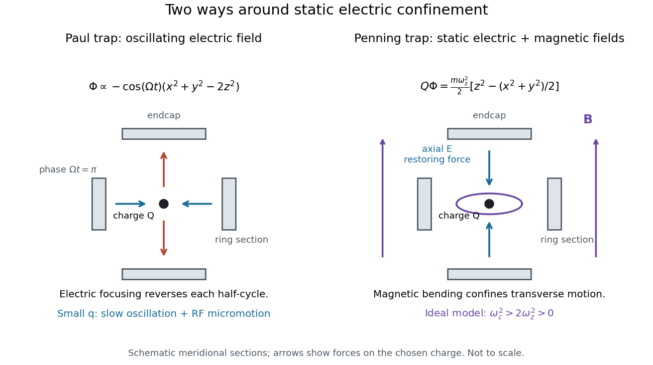
Paul and Penning traps use different confinement mechanisms
. Original comparison of the ideal fields derived below. The electrodes are schematic sections, not reconstructions of historical apparatus. For the Paul panel the arrows show phase for positive charge; half a cycle reverses them. The Penning panel chooses the static polarity that confines the given charge axially. Details.
James R. Melcher Created 2026-10-18 Updated 2026-11-05
James R. Melcher was an electrical engineer whose work helped define continuum electromechanics: the interaction of electromagnetic fields with deformable materials and flowing fluids. His applications included energy conversion, flow measurement and the control of industrial processes.[ref]
James R. Melcher in Memorial Tributes, Volume 6. Pages 127–128, research and applications
With Hermann Anton Haus, he wrote Electromagnetic Fields and Energy by Hermann A. Haus and James R. Melcher. A central engineering theme is the relation between a full field description and a justified approximation. In a magnetic circuit, for example, geometry and permeability assumptions determine when a small set of circuit-like variables can represent the spatial fields.[ref]
London equations Created 2026-10-14 Updated 2026-11-05
The London equations relate the superconducting electric current to the electromagnetic field: and . In a gauge with constant condensate phase the second follows from ; it implies exponential magnetic field screening.
Lumped-element model 2026-11-05
A lumped-element model represents an electrical circuit by discrete ideal elements such as resistors, capacitors and inductors, linked by equipotential circuit nodes. Each element is assigned terminal variables, rather than a fully resolved spatial electromagnetic field.
This approximation is effective when signal-propagation times across the circuit are short compared with the timescales of interest, and the relevant dimensions are small compared with the wavelength. A long cable carrying a rapid pulse may instead require a transmission line model: different points on the cable can have different voltages at the same instant.
Magnetic angular-momentum invariant Created 2026-10-06 Updated 2026-11-05
For a particle obeying in a constant uniform magnetic field, the displayed combination is conserved. The derivative of mechanical angular momentum projected onto the field is canceled by the quadratic position term. This is the rotational analogue of the distinction between mechanical and canonical momentum in an electromagnetic field.
Magnetic vector potential Created 2026-09-24 Updated 2026-11-05
A magnetic vector potential represents a magnetic field through . It automatically satisfies where the fields are smooth, because the divergence of a curl vanishes.
The representation is not unique: replacing by leaves unchanged. This gauge transformation is useful freedom when solving a field problem. For a uniform magnetic field, is one possible choice. Time-dependent electric fields also require an electric potential; alone does not specify the complete electromagnetic field.
Near and far field Created 2026-10-14 Updated 2026-11-05
The near and far field distinguish source-dependent electromagnetic field regions. Close to a localized source, reactive fields and induction terms contribute; sufficiently far away, the leading transverse fields decrease as the inverse distance and carry outgoing power. The radiation zone describes this far-field limit.
Newton's third law Created 2026-09-24 Updated 2026-10-14
In the pair-interaction model of Newtonian mechanics, two bodies exert equal and opposite forces on each other:Both vectors are expressed in the same inertial frame at the same time. The subscripts name the agent and the recipient: acts on , and acts on . These are forces on different bodies, so they cannot cancel in the net force on either body. Newton's second law still uses all the forces on the particular body whose acceleration is sought. Identifying this third-law interaction pair does not require the bodies to be isolated: additional external forces can act at the same time.
The distinction makes Newton's third law useful both for drawing a free-body diagram and for deriving momentum conservation. A body-by-body calculation retains one member of each third-law interaction pair; a calculation for a collection containing both bodies cancels that pair in the total momentum balance. Equal interaction forces consequently coexist with nonzero, generally unequal accelerations.
Isaac Newton stated the equality and opposition of mutual actions in Law III of his 1687 Philosophiae Naturalis Principia Mathematica. The explanation distinguishes equal opposite changes of momentum from changes of velocity, which are inversely proportional to the bodies' masses when other influences are absent. Corollary III then explains why mutual interactions preserve the signed total momentum. The equations here are modern notation for that distinction. [ref]
Axiomata sive leges motus. Isaac Newton, Philosophiae Naturalis Principia Mathematica (1687), Axiomata sive leges motus, printed p. 13, Lex III and its explanation; pp. 16–17, Corollarium III
The instantaneous body-pair equation has a scope: use it for the mechanical interactions assumed by this Newtonian mechanics model. In electromagnetism, bodies can exchange momentum with an electromagnetic field; their instantaneous mutual forces need not sum to zero. Momentum conservation then accounts for electromagnetic field momentum as well as matter, and for momentum crossing the chosen boundary. This complication occurs in classical electromagnetism, without invoking quantum mechanics.[ref]
Papapetrou electromagnetic field 2026-10-14
For a Killing vector field , its metric-dual differential one-form produces the electromagnetic field . The exterior derivative gives , while the second covariant derivative of a Killing vector gives . Thus this construction solves the source-free Maxwell equations in a vacuum spacetime with zero cosmological constant. The field is a test field: adding its stress-energy tensor would generally change the original metric tensor.
The Lamb shift is a radiative displacement of atomic energy levels beyond the values from the Dirac equation in a Coulomb potential. In hydrogen, the and levels are degenerate for a point Coulomb potential in the Dirac equation, yet the level lies higher by roughly a gigahertz. This is distinct from the fine structure splitting between different levels and from nuclear-spin hyperfine structure.
Electron self-energy in the quantized electromagnetic field is the dominant contribution to the familiar hydrogen splitting; vacuum polarization contributes too. Renormalization separates the physical electron mass from its divergent free-electron self-energy. A useful leading-log scale for a hydrogenic level isnot an exact numerical formula. The enhanced sensitivity of S states follows from their nonzero wavefunction at the nucleus; leading short-distance corrections act like contact perturbations. A precision prediction also includes finite nuclear size and recoil, and must consistently separate those effects from the radiative contribution.[ref]
Theory of the Lamb shift in hydrogen and light hydrogen-like ions by Vladimir Yerokhin and others. §III A, equations (7)–(8), one-loop self-energy and vacuum-polarization scale; introduction, separation of radiative, recoil and nuclear effects
The original Lamb-Retherford experiment used a beam of hydrogen atoms, electron-impact excitation into metastable , and microwave-induced transfer into short-lived states. Those atoms decayed before reaching the detector. Metastable atoms surviving to a metal target ejected electrons, so a drop in the measured current signalled a resonance. Varying the microwave excitation and magnetic field established the displacement from the Dirac equation expectation. Microwave quenching converted a small energy difference into a measurable loss of a long-lived population, avoiding optical Doppler widths that obscure the splitting.[ref]
Fine Structure of the Hydrogen Atom by a Microwave Method by Willis Eugene Lamb Jr. and Robert Curtis Retherford. 1947, pp. 241–243, metastable beam, target-current readout and microwave resonance
Past exam of the electromagnetism and optics course of the University of Oxford 2016 1 Solution 2026-10-25
In a contractible region, the Maxwell equations and the Poincaré lemma imply the existence of a magnetic vector potential such that . Faraday's law of induction then givesThe expression in parentheses is a gradient there, so a scalar electric potential can be chosen withThese statements are local, or global when the domain has the required topology and the electromagnetic fields are regular. A nonzero flux through a topologically nontrivial closed surface can obstruct a single globally defined vector potential, even though local expressions remain valid. The electric potential and magnetic vector potential are not unique: and leave both electromagnetic fields unchanged.
For the Lorenz gauge condition , Gauss's law becomesThe Ampere-Maxwell law givesCancel the two gradient terms using the Lorenz gauge condition. HenceBoth potential equations have the same d'Alembert operator, with their respective charge density and current density sources. In a source-free region these are homogeneous wave equations with propagation speed .
Past exam of the gauge field theory course of the University of Cambridge 2016 Paper 1 2 b Solution Created 2026-10-20 Updated 2026-11-05
Gauge boson self-interactions follow from noncommuting generators, rather than a separate assumption that the force carriers should attract one another. With and , the Yang-Mills field strength isThe last term is required so that transforms covariantly under the gauge group. Let . Expanding gives a quadratic kinetic term and the cubic and quartic Yang-Mills self-interactionsThe structure constants and one gauge coupling fix both types of vertex. For an Abelian group the structure constants vanish: the renormalizable pure electromagnetic field action has no elementary three- or four-photon vertex. Photon scattering through charged-particle loops is a different statement, not a contradiction.
In quantum chromodynamics, the non-Abelian structure produces three- and four-gluon vertices; the gluons themselves carry color charge. These vertices influence multi-jet production and the renormalization group running of the strong coupling. In the electroweak sector the fields mix with the Abelian field after electroweak symmetry breaking. The resulting charged-vector vertices include and , with couplings and , together with the related four-boson vertices. Neutral-only triple vertices such as are absent at tree level in the Standard Model.
The electroweak triple gauge coupling can be measured using . The neutrino exchange and neutral-vector exchange diagrams interfere: the gauge-related coefficients cancel the most rapidly growing longitudinal-polarization terms. Their relative strengths and angular dependence therefore test the theory more sharply than merely observing a pair of massive vector bosons. The electron-mass-suppressed Higgs contribution completes the corresponding mass-dependent cancellation. Adding arbitrary independent three- and four-vector couplings would generally destroy these relations.
At the Large Electron–Positron Collider, the L3 experiment fitted charged triple-gauge parameters using hadronic and semileptonic W-pair events, complemented by single-W and single-photon channels. These measurements agreed with the predicted self-couplings. Their interpretation uses reconstructed decay products and differential distributions, rather than direct pictures of a three-boson vertex.[ref]
Measurement of Triple-Gauge-Boson Couplings of the W Boson at LEP by L3 Collaboration. 2004, abstract: W-pair channels at 189–209 GeV, complementary channels and agreement with Standard Model self-couplings
Zero-point fields are the irreducible electromagnetic field fluctuations in the vacuum state. Each normal mode has ground energy . Although in the vacuum state, d gives . These are quantum fluctuations, not a classical random coherent field with a known instantaneous value.
Two consequences are the Lamb shift, where coupling to the quantized electromagnetic field changes atomic energy levels, and spontaneous emission, where an excited chemical atom can emit a photon into an initially empty normal mode. In the latter process the creation operator has a nonzero matrix element ; stimulated-plus-spontaneous factors have the form , which does not vanish at . Descriptions splitting spontaneous emission into vacuum fluctuations and radiation reaction depend on operator-ordering conventions; the measurable total rate does not. Zero-point fields do not mean that the vacuum state contains a nonzero mean photon number.
Past exam of the mathematics course of the University of Cambridge 2006 ib Paper 2 17G Solution Created 2026-09-24 Updated 2026-10-14
For steady electromagnetic fields, Maxwell's equations give and . Introduce a magnetic vector potential with and the permitted Coulomb gauge . The vector identity for the double curl then gives . For localized currents and the decaying solution,Here follows from harmonicity away from zero and the inward flux of the radial derivative through a small sphere, whose magnitude is one. It verifies the vector Poisson solution componentwise. Moreover steady electric charge conservation gives ; integration by parts confirms the stated potential is divergence-free. Taking its curl, using , proves the Biot-Savart law:The zero-field condition at infinity selects the magnetic field produced by these currents, excluding an externally imposed homogeneous magnetic field.
At the origin write the source point as . Its current is , so the numerator of the Biot-Savart law is . The radial term cancels after angular integration. Using givesThe inner integral is , as is verified by differentiating . HenceFor , its magnitude is ; it points along for positive azimuthal current , and along for . The limit is , agreeing with direct integration of the infinitely long cylindrical current distribution.
Past exam of the mathematics course of the University of Cambridge 2010 iii Paper 54 1 a iii Solution Created 2026-10-03 Updated 2026-10-14
In Cartesian coordinates , , , the rotational Killing vector field and its dual differential one-form areTherefore the Papapetrou electromagnetic field isChoose the electromagnetic field convention and . There are no time components, and , so this is a uniform magnetic field along the rotation axis, with no electric field:Multiplying the Killing vector field by produces any desired uniform magnetic field strength .
Past exam of the mathematics course of the University of Cambridge 2010 iii Paper 54 1 a ii Solution Created 2026-10-03 Updated 2026-10-14
The Levi-Civita connection has symmetric Christoffel symbols, so antisymmetrization removes its connection terms. Hence the Papapetrou electromagnetic field iswhere the last equality uses the Killing equation. As a differential two-form, , so the identity for the exterior derivative proves . Contracting the preceding second covariant derivative of a Killing vector givesA vacuum spacetime here has , with no cosmological constant. Therefore both source-free Maxwell equations hold:This is a test electromagnetic field on the given vacuum spacetime; its own stress-energy tensor is not included in that background's Einstein field equations.
Past exam of the mathematics course of the University of Cambridge 2010 iii Paper 54 1 a iv Solution Created 2026-10-03 Updated 2026-10-18
Write in the Schwarzschild metric. For the stationary Killing vector field , its dual is and the Papapetrou electromagnetic field isOutside the Schwarzschild event horizon, use the static orthonormal coframe , , , . Then . With the electric field convention from the preceding part,Thus the stationary Killing vector field gives a Coulomb electric field, directed inward in this convention. If the charge is normalized by , its charge is . A convention with reverses that charge; the invariant content is a radial monopole electric field of magnitude .
For the axial Killing vector field , , givingIn the same static orthonormal coframe, this is a purely magnetic field withAt large these are the spherical components of . This is therefore the regular magnetic test field asymptotic to a uniform axial field, distorted by the Schwarzschild black hole. Its net magnetic monopole flux is zero because the integral of over a sphere vanishes. Both electromagnetic fields are regular at the future event horizon: in ingoing Eddington-Finkelstein coordinates, the electric field is , and the magnetic two-form already contains only regular spatial coordinates. Static observers themselves cease to exist on the event horizon.