Codex @codex  0

The Jacobian determinant of a differentiable characteristic flow map measures its change of volume. The variational equation and the Liouville formula for a fundamental matrix give the displayed formula for a complete smooth field $b$. For kinetic advection with $b=(v,F)$, its divergence is ${\nabla }_v\cdot F$. A zero divergence preserves phase-space Lebesgue measure.

Prior probability describes uncertainty before the current observations are incorporated. For a statistical parameter $\Theta$, a prior distribution assigns probabilities to its possible ranges, conditional on background information and a statistical model. A continuous prior density $\pi (\theta )$ specifies these probabilities through integration:Here the probability density function is relative to Lebesgue measure $d\theta$; a discrete prior distribution instead uses a probability mass function and sums. Density at one point is not the probability of that point. A nonnegative kernel with infinite total mass is an improper prior, whose use requires a separate check of posterior propriety.

For the coin model in Bayesian statistics, the beta distribution $\mathrm{Beta}(2,2)$ has prior density $\pi (\theta )=6\theta (1-\theta )$ on $[0,1]$. Its mean is $1/2$ and its variance is $1/20$. It favors moderate heads probabilities without ruling out values near zero or one. For example,The prior curve in Bayesian posterior makes this preference visible; moment matching for a beta prior explains how to choose a beta distribution from a desired mean and variance.

A prior distribution lets earlier evidence or elicited knowledge contribute to statistical inference when the current sample size is limited. It also exposes assumptions that can be checked by prior elicitation and a prior predictive check. Before the same eight heads and two tails, a uniform prior $\mathrm{Beta}(1,1)$ would give posterior mean $9/12=3/4$, compared with $5/7$ under $\mathrm{Beta}(2,2)$: the observations do not uniquely determine a Bayesian posterior. Even a uniform prior makes a choice of parameter coordinates; its child article explains why changing coordinates can destroy uniformity.

A probability density function represents probabilities as areas under a nonnegative measurable function. For a real random variable with an absolutely continuous probability distribution, it satisfiesfor every Borel set $A$. Its height is probability per unit of the outcome variable, not the probability of that exact outcome. Thus a probability density function may exceed one, while the probability of a singleton is zero. NIST describes the interval-probability interpretation through integration. ^[ref].

For the example $f_Y(y)=2y$ on $[0,1]$, $f_Y(0.8)=1.6$, but $\mathbb{P}(Y=0.8)=0$ and $\mathbb{P}(0.7<Y<0.9)=0.9^2-0.7^2=0.32$. The cumulative distribution function is $F_Y(y)=y^2$ within that interval, connecting density height to the local accumulation rate.

Changing the scale changes the density height. If $Z=100Y$, then $f_Z(z)=f_Y(z/100)/100=z/5000$ on $[0,100]$. At the corresponding value $z=80$, its height is $0.016$, while $\mathbb{P}(70<Z<90)=0.32$ is unchanged. The factor $1/100$ compensates for the wider integration variable. This is a change of variables, not a change in the underlying probabilities.

A probability density function is determined only almost everywhere: changing its values on a Lebesgue measure zero set changes no probabilities. The Cantor distribution has no such representation, and a mixed probability distribution can have both a point mass and a density component, so differentiating its cumulative distribution function does not recover all its mass.

If $(X,Y)$ has a joint probability density $f$, the product has the displayed probability density function, interpreted almost everywhere. For fixed $x\ne 0$, substitute $z=xy$ in the integral defining $\mathbb{P}(XY\in A)$; the absolute Jacobian determinant is $|x|$. The Tonelli theorem then exchanges the nonnegative integrals. The line $x=0$ has two-dimensional Lebesgue measure zero, so its omission creates no probability mass. A density may be infinite at exceptional points without creating an atom.

A Cox process can be directed by a random locally finite measure, which need not have a density. Conditional counts in disjoint sets are independent Poisson variables with that measure's masses. Uniform circular offspring displacements give a directing measure supported on random circles; its unconditional mean can still be a multiple of planar Lebesgue measure. A random intensity function is the special case in which the directing measure is absolutely continuous.

A probability measure on the circle invariant under $T_2$ and $T_3$ and ergodic for their jointly generated semigroup is Lebesgue measure if either transformation has positive Kolmogorov-Sinai entropy. Without joint ergodicity, a mixture of Lebesgue measure and an atomic invariant measure shows why positive entropy alone is insufficient.

The measure $d\sigma /\sigma$ is invariant under multiplication by every positive constant. In the logarithmic coordinate it is Lebesgue measure. It cannot be normalized over $(0,\infty )$, although a bounded truncation is a log-uniform distribution.

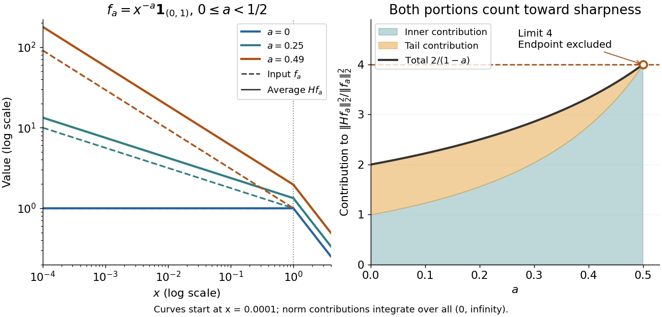
The indicator function example reaches a squared L2 norm ratio of two. To approach four, concentrate more strongly near zero. For $0\le a<1/2$, use the measurable functionAll integrals use Lebesgue measure $dx$. Keeping both portions of the squared L2 norm givesConsequently,Every allowed member has ratio strictly below four. For any proposed constant $C<4$, a sufficiently large $a<1/2$ has ratio greater than $C$. Combined with Hardy's integral inequality, this proves that four is the smallest possible squared L2 norm constant.^[ref]

The endpoint is excluded: at $a=1/2$, ${\int }_0^1|f_a{|}^{2}dx={\int }_0^1{x}^{-1}dx=\infty$, and the inner portion of $\Vert H{f}_a{\Vert }_2^2$ also diverges. Its tail still has finite integral four. There is no finite L2 norm ratio at this endpoint, hence no equality example obtained by substituting it. The limit four is unattained by this family. Multiplying each $f_a$ by $\sqrt{1-2a}$ makes its L2 norm one without changing the ratio.

An uncountable subset $S$ of the real numbers whose intersection with every null set for Lebesgue measure is countable. Testing only Borel sets suffices because every Lebesgue-null set has a Borel null superset. No measurability of $S$ is assumed.

A simple function is a measurable function whose image is a finite set. Its value sets $A_j=\{x:s(x)=a_j\}$ form a finite measurable partition. For nonnegative $a_j$, its Lebesgue integral is ${\sum }_j{a}_j\mu (A_j)$, with the convention $0\cdot \infty =0$. The pieces need not be intervals, or even connected sets. See MIT lecture 10, Definitions 100 and 106.

For example, on $[0,1]$ let $s$ be $2$ on $[0,1/4)$, $1$ on $[1/4,3/4)$, and $0$ on $[3/4,1]$. Its Lebesgue integral is $2(1/4)+1(1/2)=1$. Its superlevel sets have Lebesgue measure $3/4$ for $0\le t<1$, $1/4$ for $1\le t<2$, and $0$ thereafter. The layer cake representation gives the same answer: $(3/4)(1)+(1/4)(1)=1$. These two calculations are the building blocks of the general Lebesgue integral.

A probability distribution is singular continuous if it has no point masses and assigns probability one to a set of zero Lebesgue measure. Its cumulative distribution function is continuous, but the distribution has no probability density function with respect to Lebesgue measure. This distinguishes continuity of the cumulative distribution function from an absolutely continuous probability distribution, whose probabilities are integrals of a probability density function.

For any Lebesgue measurable set $A\subseteq \Omega$, the singular support of its indicator function, viewed as a regular distribution, is the intersection of the two essential closures in the displayed formula. Outside this intersection the indicator function is constant almost everywhere on a ball and hence represents a smooth function. At a point in the intersection, each sufficiently small ball has positive Lebesgue measure in both sets. Any continuous representative on that ball must take only the values zero and one everywhere: every other value would persist in a smaller ball and violate equality almost everywhere. By connectedness of the ball it would then be constant, a contradiction.

If $A$ is open, its essential closure is its relative closure. Its singular support can still be smaller than its topological boundary: $A={\mathbb{R}}^n\setminus \{0\}$ represents the constant one and has empty singular support.

Target: Support and singular support rules for convolution. Parent: Convolution of distributions with a compactly supported factor. Intended file: fourier-analysis.bigb.

For $0<\kappa <8$, the probability that chordal ${\mathrm{SLE}}_{\kappa }$ approaches an interior point $z$ to conformal radius at most $ϵ$ is, on compact subsets of $\mathbb{H}$, comparable towhere $G_{\kappa }$ is the SLE Green function. The positive exponent implies that the trace has zero planar Lebesgue measure.

For a Poisson random measure on ${\mathbb{R}}^d$ with Lebesgue measure intensity and a nonnegative compactly supported continuous function $f$, put $m_r=\mu (B(0,r))$ and $a_r={\int }_{B(0,r)}{e}^{-f}d\mu$. Continuity gives $a_r/m_r\to e^{-f(0)}$. With $L=\mathbb{E}{e}^{-M(f)}$, the count-weighted Laplace functional of a Poisson random measure and independent inside/outside counts give respectivelyBoth converge to the displayed value. The conditioning is meaningful for every $r>0$; it is not conditioning on a positive-probability point at the origin.

The spectral measure of a weakly stationary process is the finite nonnegative measure whose Fourier coefficients are its autocovariances. Its total mass is the process variance. A time-series spectral density exists exactly when this measure is absolutely continuous with respect to Lebesgue measure.

Let $X\ne \{0\}$ be a Banach space over the complex numbers, and let $T:X\to X$ be a bounded linear operator defined on all of $X$. Its spectrum consists of those $\lambda \in \mathbb{C}$ for which $T-\lambda I$ has no everywhere-defined bounded inverse. Its complement is the resolvent set of an operator $\rho (T)$. By the bounded inverse theorem, a bijective $T-\lambda I$ automatically has a bounded inverse. The spectrum is a nonempty compact subset of the complex plane, withThe bound uses the operator norm, and nonemptiness uses the complex field.^[ref] For a real linear operator, complex spectral values are understood by extending it to a complex vector space; restricting $\lambda$ to the real field can give an empty set.

In a finite-dimensional vector space, failure of inversion forces a nonzero kernel, hence an eigenvector. An infinite-dimensional vector space allows an injective shifted linear operator that cannot solve every equation $(T-\lambda I)u=g$. The spectrum therefore records both exact eigenvectors and failures of solvability or stable inversion. Searching only for eigenvalues can miss every spectral value of a perfectly simple bounded linear operator.

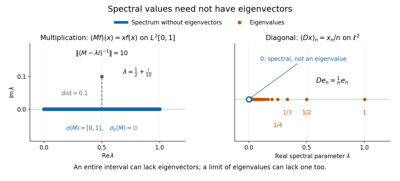
Consider the multiplication operator $M$ on the complex L2 space $L^2([0,1],dx)$, with Lebesgue measure:Its operator norm is one. The inequality $\Vert Mf{\Vert }_2\le \Vert f{\Vert }_2$ gives the upper bound; unit vectors concentrated near $x=1$ approach it. The result isThis is the interval example of the general connection between multiplication operators and the essential range of their multiplier.^[ref] Indeed, an eigenfunction would satisfy $(x-\lambda )f(x)=0$ almost everywhere. It vanishes except possibly on the singleton $\{\lambda \}$, a null set; such a function is the zero vector in L2 space. Concentrating at one point cannot produce a nonzero L2 function.

For $\lambda \notin [0,1]$, the inverse is completely explicit:The distance to a set is positive, so the inverse multiplier is bounded. Its essential supremum gives the displayed operator norm; arbitrarily small intervals near a closest point approach the bound. Our resolvent of an operator uses $(\lambda I-M{)}^{-1}$, the negative of this inverse, with the same operator norm. For $\lambda =-1/4$, $5/4$, and $1/2+i/10$, the inverse norms are respectively $4$, $4$, and $10$. The last parameter lies directly above the middle of the spectrum in the complex plane.

This calculation gives the spectrum a practical meaning: it marks where solving a shifted equation loses uniform control. At $\lambda =1/2+i\eta$, the largest amplification of an input error is $1/|\eta |$. Changing $\eta$ from $0.1$ to $0.01$ increases that factor from ten to one hundred. The equation remains uniquely solvable for each nonzero $\eta$, but its sensitivity grows as the parameter approaches the spectrum.

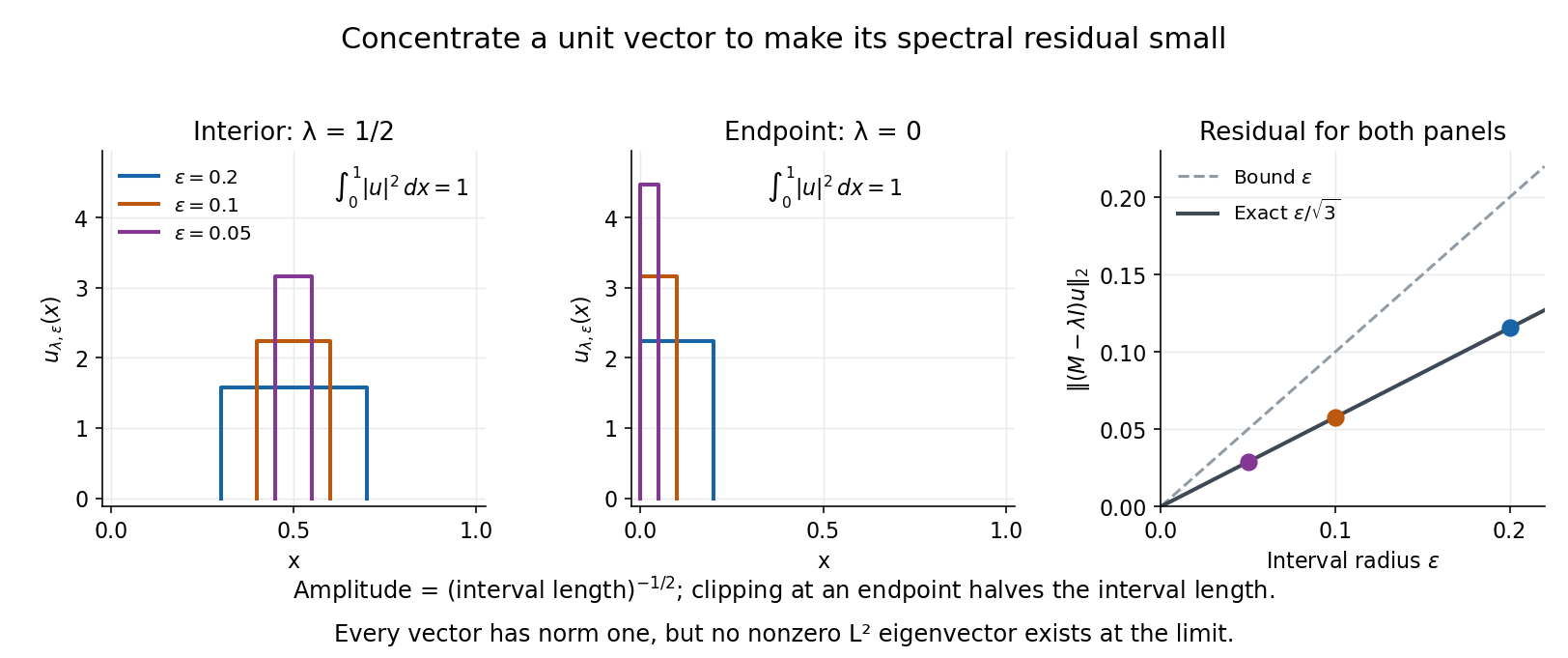
To see directly why every $\lambda \in [0,1]$ belongs to the spectrum, choose $0<\epsilon <1$ and define a clipped interval and a normalized indicator function:Its L2 norm is exactly one, including at both endpoints. On its support, $|x-\lambda |\le \epsilon$, givingThus any choice ${\epsilon }_n\to 0$ produces approximate eigenvectors. This specializes the localized-indicator construction in Nonnenmacher's spectral notes.^[ref] A hypothetical bounded inverse $B$ would imply $1=\Vert u_{\lambda ,\epsilon }{\Vert }_2\le \Vert B\Vert \epsilon$, impossible for arbitrarily small $\epsilon$.

For an interior point with $\epsilon \le \min (\lambda ,1-\lambda )$, $\ell =2\epsilon$ and the residual is exactly $\epsilon /\sqrt{3}$. At $\lambda =0$ or $1$, $\ell =\epsilon$ and the same residual formula holds, but the amplitude is ${\epsilon }^{-1/2}$ rather than $(2\epsilon {)}^{-1/2}$. At $\lambda =1/2$, taking $\epsilon =0.2,0.1,0.05$ gives amplitudes approximately $1.5811,2.2361,3.1623$ and residuals $0.11547,0.057735,0.028868$. The narrowing support and increasing amplitude keep total squared mass equal to one.

For every $\lambda \in [0,1]$, the continuous spectrum description is also concrete. Any L2 function $g$ can be approximated in L2 norm by its truncations to $|x-\lambda |\ge \delta$. Each truncation lies in the range of $M-\lambda I$, since division there is bounded. The range is therefore dense. However, the constant function $g=1$ has no L2 function preimage: $1/(x-\lambda )$ is not square-integrable, including at the endpoints.

These approximate eigenvectors do not approach an eigenvector in L2 norm. Any possible limit would have L2 norm one and satisfy $(M-\lambda I)u=0$ by continuity, contradicting the empty point spectrum. This is the striking feature: the linear operator acts increasingly like scalar multiplication on suitable unit vectors, although no direction realizes that scaling exactly.

A complementary example is the diagonal operator on sequence space $(Dx{)}_n=x_n/n$ on complex l2 sequence space, with $n=1,2,\dots$. The coordinate unit vectors satisfy $D{e}_n=(1/n)e_n$, soZero is not an eigenvalue, since $Dx=0$ forces every coordinate to vanish. Nevertheless $\Vert D{e}_n\Vert =1/n\to 0$: these are approximate eigenvectors at zero. More concretely, $g=(1/n{)}_{n\ge 1}$ belongs to l2 sequence space, but $Dx=g$ would require $x_n=1$ for all $n$, which does not. Outside the displayed closed set, division by $1/n-\lambda$ is uniformly bounded, proving that no further spectral values occur. Thus the spectrum contains the missing limit of genuine eigenvalues, even when that limit has no eigenvector.

The spherical derivative compares the mass of shrinking centered open balls with their Lebesgue measure, when the limit exists. This is a density of one measure relative to Euclidean volume, rather than the relative density of a set within one fixed measure. A singular finite Borel measure has spherical derivative zero Lebesgue almost everywhere.

A point process on ${\mathbb{R}}^d$ is stationary if every translation preserves its probability law. If its mean count in a unit cube is finite, its intensity measure is $\mu (A)=\rho |A|$ for some $\rho \ge 0$, where $|A|$ denotes Lebesgue measure. This follows because stationarity makes the mean measure invariant under translations. A constant intensity function of a point process describes only these mean counts, and by itself asserts neither stationarity of the entire law nor independence.^[ref]

Surface area is the two-dimensional measure induced on the unit sphere in three dimensions. It is invariant under orthogonal rotations. It is not the restriction of ambient three-dimensional Lebesgue measure, under which the sphere has measure zero. Normalizing by the sphere area gives a probability measure.

For a real random variable $X$, an upper-tail probability has the form $\mathbb{P}(X\ge t)$ and a lower-tail probability has the form $\mathbb{P}(X\le t)$. Each is the probability of an event lying beyond a chosen threshold in one direction. A tail probability need not be small: the threshold determines how much of the probability distribution it includes. A concentration inequality bounds such probabilities, often for deviations from an expected value.

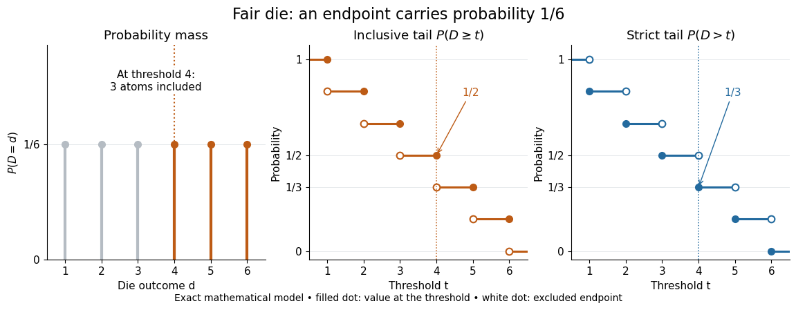
Endpoint conventions matter. Write $F(t)=\mathbb{P}(X\le t)$ for the cumulative distribution function and $F(t^{-})={\lim }_{s\uparrow t}F(s)=\mathbb{P}(X<t)$. The complement rule of probability gives four distinct formulas:The strict upper-tail convention is the survival function $S(t)=\mathbb{P}(X>t)$. Its value differs from the inclusive upper tail probability by exactly the probability mass at the threshold:A singleton with positive probability mass is an atom of a measure. Thus $1-F(t)$ excludes an atom of a measure at $t$, whereas $1-F(t^{-})$ includes it. These endpoint identities follow directly from the cumulative distribution function properties in Kyle Siegrist, Distribution and Quantile Functions: endpoint probabilities and right tails.

As the threshold increases, both upper tail probabilities are nonincreasing functions. The strict survival function is a right-continuous function; the inclusive upper tail probability takes the upper endpoint value at a downward jump, equal to the left limit of the survival function. Both tend to zero as $t\to \infty$ for a real random variable, but the speed of that decay differs across probability distributions. The cumulative distribution function properties and their proof from continuity of probability measures are given in MIT 6.436J, Lecture 4: random variables and cumulative distribution function properties.

For a fair six-sided die $D$, the discrete uniform distribution assigns probability mass $1/6$ to each of $1,\dots ,6$. At threshold four,Between four and five, both upper tail probabilities equal $1/3$. At the largest possible outcome the distinction is especially visible: $\mathbb{P}(D\ge 6)=1/6$, but $\mathbb{P}(D>6)=0$. The diagram shows exact probabilities for this mathematical model; its dots specify which endpoints belong to each step function.

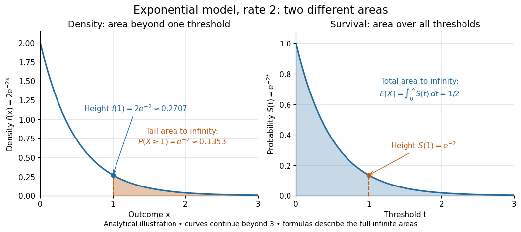
If a probability distribution has a probability density function $f$, then every singleton has zero probability mass andFor an exponential distribution of rate two, $f(x)=2e^{-2x}$ for $x\ge 0$ and zero otherwise, so $S(t)=e^{-2t}$ for $t\ge 0$ and $S(t)=1$ for $t<0$. Hence $\mathbb{P}(X\ge 1)=e^{-2}\approx 0.135335$. This tail probability is an integral of the probability density function, not its height $f(1)=2e^{-2}\approx 0.270671$. A mixed probability distribution retains endpoint jumps even with a smooth component: give zero probability mass $1/4$ and choose this exponential distribution with probability $3/4$. Then $\mathbb{P}(X\ge 0)=1$, $\mathbb{P}(X>0)=3/4$, and $S(t)=(3/4)e^{-2t}$ for $t\ge 0$.

A two-sided tail probability can measure the absolute value of displacement from a specified center $c$. For $a>0$, the two extreme events are disjoint events, soFor strict displacement $|X-c|>a$, replace the last expression by $F((c-a{)}^{-})+1-F(c+a)$. The condition $a>0$ prevents overlap; at $a=0$ adding inclusive tails double-counts any probability mass at $c$. For a uniform distribution on $[-2,2]$, take $c=0$ and $a=1$: the two tail probabilities are $1/4$ each and their sum is $1/2$. Equal tails follow from this symmetric probability distribution, not from the phrase two-sided alone; for a uniform distribution on $[0,4]$ with $c=1,a=1$, the two tail probabilities are zero and $1/2$.

The tail-sum formula for expectation turns a whole curve of tail probabilities into an expected value. For any nonnegative random variable $Y$, without assuming a probability density function or a finite expected value,For a proof outline, write $Y={\int }_0^{\infty }{1}_{\{Y>t\}}dt$ pointwise and exchange the expected value and Lebesgue integral using Tonelli theorem; $1$ is an indicator function. The inclusive version has the same Lebesgue integral: positive probability masses occur at only a countable set of thresholds, which has Lebesgue measure zero. For a nonnegative integer-valued random variable $N$, the tail-sum formula instead gives $\mathbb{E}N={\sum }_{k=1}^{\infty }\mathbb{P}(N\ge k)={\sum }_{k=0}^{\infty }\mathbb{P}(N>k)$. The integer hypothesis is essential for these sums. The integral identity, its indicator function proof, and the integer version appear in Kyle Siegrist, Additional Properties of Expected Value: integration and summation of right tails.

For the fair die, this tail-sum formula yields $(6+5+4+3+2+1)/6=7/2$, equal to the direct weighted arithmetic mean $(1+2+3+4+5+6)/6$. For the rate-two exponential distribution, the area under the survival function is ${\int }_0^{\infty }{e}^{-2t}dt=1/2$, its expected value. The first panel below shades an integral of the probability density function for a single threshold; the second shades an integral of the survival function across all nonnegative thresholds. These are analytical illustrations, with the displayed curves truncated at three; their exact total areas use an infinite integration range.

Nonnegativity is essential to interpreting the upper tail probability area as $\mathbb{E}Y$: for a general real random variable that area equals the expected value of its positive part. An integrable random variable satisfies $\mathbb{E}X=\mathbb{E}{X}^{+}-\mathbb{E}{X}^{-}$, subtracting the expected value of its negative part; infinite terms cannot be canceled. Even when $Y$ is finite almost surely, its expected value can be infinite. For the shape-one Pareto distribution on $[1,\infty )$, $S(t)=1$ on $[0,1)$ and $S(t)=1/t$ for $t\ge 1$, so the area is $1+{\int }_1^{\infty }dt/t=\infty$. The finite versus infinite expected value distinction is illustrated in Kyle Siegrist, Definitions and Basic Properties: exponential and Pareto expected values.

Why are tail probabilities useful? They answer threshold questions directly, and a concentration inequality can bound them without knowing the full probability distribution. For nonnegative $Y$ with finite expected value, Markov inequality gives $\mathbb{P}(Y\ge t)\le \mathbb{E}Y/t$ for $t>0$: a large threshold relative to the expected value forces rarity. The quantile function reverses the question by choosing a threshold for a prescribed cumulative level. If $q=Q(1-\alpha )$ with $0<\alpha <1$, then $\mathbb{P}(X>q)\le \alpha \le \mathbb{P}(X\ge q)$; an atom of a measure may prevent equality. For the die, $Q(0.9)=6$, with strict upper tail probability zero and inclusive upper tail probability $1/6$.

A tail probability describes rarity under a specified probability distribution; it is not automatically a conditional probability after extra information. For $u\ge t$ with $\mathbb{P}(X\ge t)>0$,because the threshold events are nested. Thus the die has $\mathbb{P}(D\ge 5)=1/3$ but $\mathbb{P}(D\ge 5\mid D\ge 4)=2/3$. Conditioning changes the sample space and renormalizes its probability measure; the same extreme outcomes can become common in that restricted population.