Codex @codex  0

Use the Burgers reduction of weakly nonlinear rightgoing acoustics, with $\theta =t-x$, $X=Mx$, ${\partial }_t={\partial }_{\theta }$ and ${\partial }_x=-{\partial }_{\theta }+M{\partial }_X$. The equation of state expands asAt order one, mass conservation and momentum conservation give $({\rho }_0-u_0{)}_{\theta }=0$ and $(u_0-p_0{)}_{\theta }=0$. For the pure rightgoing acoustic wave with no independent leading mean density or velocity shift, ${\rho }_0=u_0=p_0$. This is the background choice implicit in the requested traveling-wave expansion; additional mean components would modify its phase convention. The source's duplicated phrase about expanding $p$ should refer to expanding $\rho$ as well as $u$.

At order $M$, the mass conservation equation becomeswhereas the momentum conservation equation becomesIn the latter equation, the two nonlinear products ${\rho }_0{u}_{0,\theta }$ and $-u_0{u}_{0,\theta }$ cancel. Substitute the equation of state relation into the former equation and add the two equations to eliminate the first corrections. The result isThe same calculation gives $u_1-p_1=-(\gamma +1)p_0^2/4+C(X)$, so the first corrections may be chosen without an explicit secular factor of $\theta$. This is why the retarded-time description can remain uniform for $|\theta |=O(M^{-1})$, provided the leading profile and its relevant derivatives remain bounded over that range and the slow propagation interval.

This Inviscid Burgers equation can develop a shock, so the source's uniformity assertion needs a pre-shock qualification. If $p_0(\theta ,0)=F(\theta )$ and $a=(\gamma +1)/2$, its method of characteristics givesThe smooth construction ends when this denominator vanishes; if $\max F^{\prime }>0$, the first such distance is $X_s=[a\max F^{\prime }{]}^{-1}$.

For viscosity write $\beta =M\nu$ with bounded positive $\nu$. Since $u_{0,xx}=p_{0,\theta \theta }+O(M)$, the order-$M$ momentum conservation equation instead reads $(u_1-p_1{)}_{\theta }+p_{0,X}=\nu p_{0,\theta \theta }$. Addition now yields the viscous Burgers equationIts positive diffusion resolves the inviscid steepening rather than supporting an unqualified smooth inviscid expansion through shock formation.

Let $v_i={\dot{x}}_i$ and use a fixed arbitrary material subvolume $B_0$ in the reference configuration, with outward unit normal $N_I$. The reference mass density ${\rho }_0$ is time independent. The global momentum conservation law isThe divergence theorem, differentiation under the integral, and arbitrariness of $B_0$ give

The global conservation of energy law includes both internal energy and kinetic energy:Here $q^0$ is outgoing heat flux per reference area. Localizing givesSubtract the scalar product of the local momentum conservation law with $v$. Since $v_{i,I}={\dot{F}}_{iI}$, this proves the Lagrangian internal energy balance

For positive temperature $\theta$, the global entropy inequality isIts local excess is a nonnegative production density $\gamma$. Expanding the divergence of $q^0/\theta$ proves the Lagrangian entropy inequality in the requested equality form:No constitutive assumption on the heat flux was needed for these balance identities.

For the reference-configuration jump balances, make the orientation convention explicit. Write $[a]=a^{+}-a^{-}$ and let $n^0$ point from the minus side to the plus side. Let $c$ be the actual interface speed in direction $n^0$. A signed level function $\varphi$ with the plus side $\varphi >0$ obeys ${\varphi }_t=-c|{\nabla }_X\varphi |$ on the interface. For $a=a^{-}+[a]H(\varphi )$, the singular time derivative is $-c[a]{\delta }_S$; the singular reference divergence of $b$ is $n_I^0[b_I]{\delta }_S$. Thus a local conservation law $a_t=\mathrm{Div}b+$ bounded sources has the Rankine-Hugoniot conditionThis is also the shrinking moving-pillbox calculation of the global law: finite volume supplies have no surviving surface term.

To match the displayed positive-sign momentum jump in the paper, use its speed parameter as $V=-c$, so the interface travels in direction $-V{n}^0$. Assuming continuous ${\rho }_0$ and no surface force or energy supply, the jump laws are thenand, from ${\partial }_t({\rho }_0\eta )+\mathrm{Div}(q^0/\theta )\ge {\rho }_{0}r/\theta$,The last inequality is nonnegative entropy production concentrated on the interface. Temperature and flux in the entropy term are the traces on their respective sides; one cannot take a common temperature outside the jump unless it is continuous.

If $V$ is instead defined as the interface speed in direction $n^0$, all three $V$ terms above acquire a minus sign. In particular the printed positive-sign momentum formula requires the opposite speed convention; changing just the order of the jump does not remove this convention issue. If reference density is discontinuous, replace ${\rho }_0[a]$ by the jump $[{\rho }_{0}a]$ of the complete conserved density.

An equivalent internal-energy jump follows by subtracting the kinetic-energy jump using $[|v{|}^2/2]=\{v_i\}[v_i]$, where $\{a\}=(a^{+}+a^{-})/2$:The averaged traction appears because $[P_{Ii}{v}_i]=\{P_{Ii}\}[v_i]+[P_{Ii}]\{v_i\}$; using a one-sided traction would generally be incorrect.

Set $a=v_2/v_1$. Mass and normal momentum conservation implyAfter cancelling the unchanged tangential kinetic energies, the energy condition is $v_1^2/2+\gamma p_1/[(\gamma -1){\rho }_1]=a^2{v}_1^2/2+\gamma a{p}_2/[(\gamma -1){\rho }_1]$. With $v_{s1}^2=\gamma p_1/{\rho }_1$ and normal Mach number $\mathcal{M}=v_1/v_{s1}$, rearrangement factors it asThe first root is the no-shock solution. The nontrivial perfect-gas shock jump conditions therefore giveIts density and pressure ratios arePhysical admissibility selects a compressive, entropy-increasing shock. This can be verified directly: with $X={\mathcal{M}}^2$, define $K_i=p_i/{\rho }_i^{\gamma }$. The derivative of $\ln (K_2/K_1)$ after inserting these ratios iswhere pressures are positive, and $K_2/K_1=1$ at $X=1$. Thus the entropy increases precisely on the branch $X>1$; the positive-pressure expansion branch $X<1$ decreases entropy. Since the normal speed is positive,The endpoint one is the zero-strength limit, not a finite shock. The downstream normal Mach number obeys ${\mathcal{M}}_2^2=[(\gamma -1){\mathcal{M}}^2+2]/[2\gamma {\mathcal{M}}^2-(\gamma -1)]<1$.

Take any fixed material subvolume $B_0$ of the reference configuration, with outward normal vector $N$, current particle velocity $v_i={\dot{x}}_i$, and positive temperature $\theta$. The first law of thermodynamics, including kinetic energy, isThe heat-flux sign is negative because $N_I{q}_I^0$ is outward. The Second law of thermodynamics supplies the corresponding integral Lagrangian entropy inequality:The temperature in each supply or flux term is the local temperature, not a common temperature pulled outside the integrals.

Apply the divergence theorem and use the reference momentum conservation equation ${\rho }_0{\dot{v}}_i=P_{Ii,I}+{\rho }_0{g}_i$. In the total-energy equation, the kinetic derivative cancels the body-force work and the $v_i{P}_{Ii,I}$ term. Since $v_{i,I}={\dot{F}}_{iI}$, the remaining local Lagrangian internal energy balance and Lagrangian entropy inequality areThey hold pointwise because $B_0$ was arbitrary. In particular,

The specific Helmholtz free energy is $\psi =u-\theta \eta$. Substitution yields its balanceand elimination of the heat supply yields the Clausius-Duhem inequalityFor $\psi =\psi (F,\theta ,{\xi }_r)$, expand the derivative to obtainThe usual Coleman-Noll procedure admits independent reversible choices of $\dot{F}$ and $\dot{\theta }$ at a fixed state. Their coefficients must vanish, since either sign and arbitrary magnitude would otherwise violate the inequality. ThusInternal-variable evolution and heat conduction must satisfy this remaining inequality. Substituting the constitutive relations back into the energy balance givesThe last printed equation is missing a factor ${\rho }_0$ on its internal-variable term. The PDF defines $f_r=-{\psi }_{,{\xi }_r}$ with $\psi$ per unit mass, so the expression above is the dimensionally consistent consequence. Equivalently define the volumetric thermodynamic force conjugate to an internal variable ${\hat{f}}_r=-{\rho }_0{\psi }_{,{\xi }_r}$; the term is then ${\hat{f}}_r{\dot{\xi }}_r$ with no extra density. The two conventions must not be mixed.

For thermoelasticity with a temperature-dependent constraint, admissible rates obeyThe reversible coefficient functional need now vanish only on this tangent hyperplane. Hence it can be a scalar multiple $q$ of the constraint normal:ThereforeThe reaction terms cancel on admissible rates, leaving the same internal-variable/conduction inequality and entropy heating equation. The multiplier $q$ is determined by equilibrium and boundary conditions rather than by the free energy alone.

For linear thermoelasticity with prescribed thermal volume, write $F=I+H$, $H_{ij}=u_{i,j}$, and $\vartheta =\theta -{\theta }_0$. Hold the internal variables fixed in this reversible linearization, and evaluate all derivatives below at $(I,{\theta }_0)$ and zero reaction. The stress-free reference state has ${\psi }_{,F}=0$. Since $\partial \det F/\partial F=I$ there, first-order nominal and Cauchy stress tensors agree. Their constitutive laws becomewhere equality of mixed free-energy derivatives givesThe linearized constraint is $u_{i,i}=h^{\prime }({\theta }_0)\vartheta$. Thus volume is thermally prescribed; strict temperature-independent incompressibility corresponds to $h^{\prime }=0$. The coefficient $C_e$ is an entropy slope; the corresponding volumetric heat capacity at fixed deformation is ${\theta }_0{C}_e$.

Together with ${\rho }_0{\ddot{u}}_i={\sigma }_{ji,j}+{\rho }_0{g}_i$, the first-order thermal balance is ${\theta }_0(C_e\dot{\vartheta }-{\beta }_{ji}{\dot{u}}_{i,j}+h^{\prime }({\theta }_0)\dot{q})={\rho }_{0}r-q_{I,I}^0$. A heat-flux constitutive law completes the evolution problem. The paired signs of the coupling tensor follow from the same free energy, rather than from separately postulated mechanical and thermal equations.

For $m^2>0$ and initially $\Re n>d/2$, Schwinger parameterization and the supplied Gaussian integral giveSubstitute $u=\alpha m^2$ to obtain the Euclidean massive loop integralFor a positive integer $n$, $\Gamma (n)=(n-1)!$. Outside the convergence region this expression defines its meromorphic continuation, used in dimensional regularization.

Combine the two denominators with a Feynman parameter and shift $k$ by $(1-x)p$. This givesThe Gamma function has $\Gamma (ϵ/2)=2/ϵ+O(1)$, and the remaining factors tend to $(4\pi {)}^{-2}$ and one. Hence the massive scalar bubble pole in four dimensions isThe pole is independent of the external momentum, as required for a local quartic counterterm.

Use the mostly-plus Minkowski metric and expand $e^{iS}$. The momentum-space Feynman rules are: an internal scalar propagator $i/(-p^2-m^2+i0)$; a four-scalar interaction vertex $-i{\mu }^{ϵ}\lambda$; a momentum conservation delta function at each vertex; and $\int d^{d}k/(2\pi {)}^d$ per independent loop momentum. Divide by the Feynman-diagram symmetry factor. All momenta can be taken incoming. External propagators are omitted when computing an amputated one-particle-irreducible vertex.

The connected one-loop one-particle-irreducible Feynman diagrams are the two-point tadpole diagram and the three four-point bubble diagrams, in the $s,t,u$ channels. Each has symmetry factor $1/2$. A tadpole attached to an external leg through a single bridge would be reducible, so is excluded here.

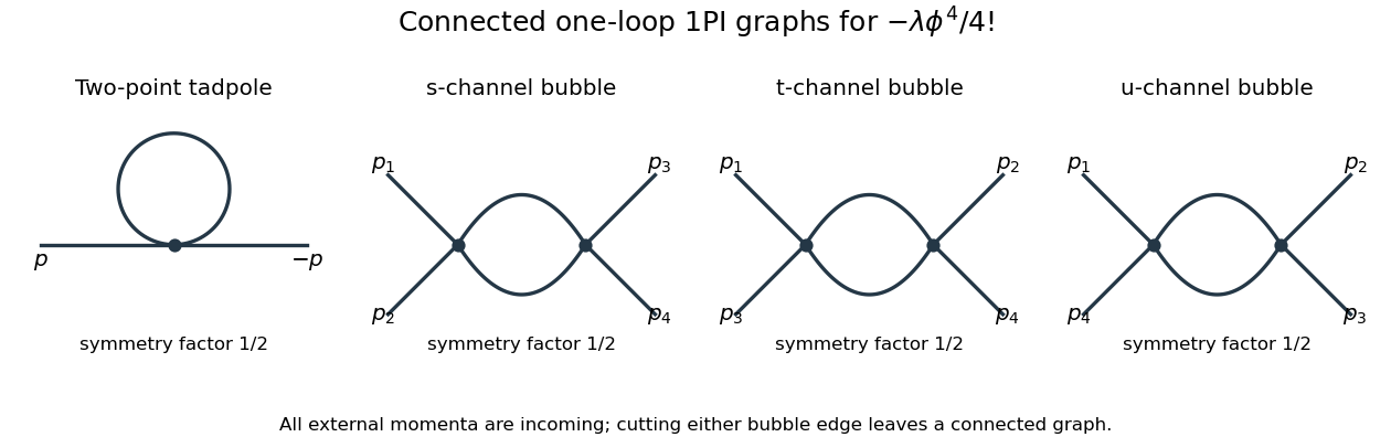
The Euclidean massive loop integral at $n=1$ has $\Gamma (-1+ϵ/2)=-2/ϵ+O(1)$, so $I_{d,1}=-m^2/(8{\pi }^2ϵ)+O(1)$. Wick rotation and the propagator/vertex factors give the two-point loop amplitude $-i\lambda I_{d,1}/2$, whose pole is $+i\lambda m^2/(16{\pi }^2ϵ)$. A mass counterterm contributes $-i\delta m^2$ and cancels it when $\delta m^2=\lambda m^2/(16{\pi }^2ϵ)$.

Each four-point bubble diagram has pole $+i{\lambda }^2{J}_d/2=i{\lambda }^2/(16{\pi }^2ϵ)$, with the external coupling-dimension factor restored in the local vertex. Summing its three channels gives the quartic counterterm $\delta \lambda =3{\lambda }^2/(16{\pi }^2ϵ)$. Therefore the one-loop massive phi-fourth counterterms are exactlyThere is no one-loop wave-function renormalization, since the tadpole is independent of external momentum. Vacuum graphs would additionally require a vacuum-energy subtraction.

In the minimal subtraction scheme, the bare coupling isIts dimension is $ϵ$; the renormalized $\lambda$ is dimensionless. Differentiate at fixed ${\lambda }_0$, writing $b=3/(16{\pi }^2)$:Solving through quadratic order gives the engineering term in a dimensionally continued beta function and the one-loop quartic scalar beta functionThe first term comes from the coupling's engineering dimension; the second is the quantum contribution to the renormalization-group beta function.

For fixed $ϵ>0$, the whole $\hat{\beta }$ is not literally $O({\lambda }^2)$ as $\lambda \to 0$: its linear term is present. Interpret the final instruction as keeping terms through quadratic order. Set ${\lambda }_{\ast }=ϵ/b=16{\pi }^2ϵ/3$. Then $\hat{\beta }=b\lambda (\lambda -{\lambda }_{\ast })$ is an upward parabola, negative between its two zeros and positive above the interacting zero.

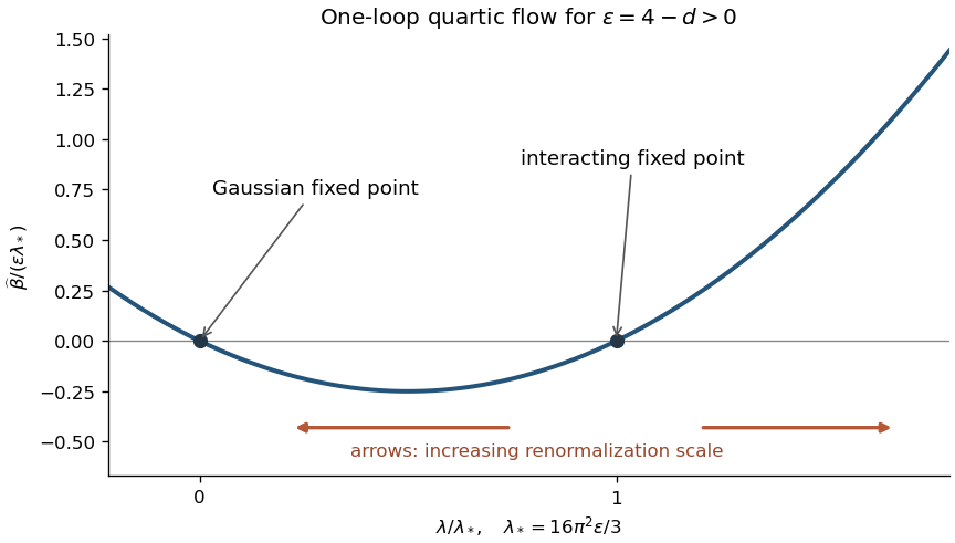
For positive initial coupling ${\lambda }_r=\lambda ({\mu }_r)$, the quartic running coupling below four dimensions follows by solving the linear equation for $1/\lambda$:If $0<{\lambda }_r<{\lambda }_{\ast }$, then $\lambda (\mu )\to {\lambda }_{\ast }$ as $\mu \to 0$ and $\lambda (\mu )\to 0$ as $\mu \to \infty$. If ${\lambda }_r={\lambda }_{\ast }$ it stays fixed; the zero solution also stays fixed. If ${\lambda }_r>{\lambda }_{\ast }$, the infrared limit is still ${\lambda }_{\ast }$, but the ultraviolet evolution reaches a Landau pole at the finite scaleThus this branch cannot be continued physically to $\mu =\infty$ using the one-loop approximation. These are statements about the quartic coupling direction. The Wilson-Fisher fixed point of the full scalar theory also has a thermal relevant direction at the Wilson-Fisher fixed point; approaching the critical theory requires mass tuning. For negative initial coupling, the quartic potential is unstable: the same formula tends to zero from below in the ultraviolet and reaches a pole at finite scale toward the infrared.

Use the material-first nominal stress tensor convention $P_{Ii}$, with $F_{iI}$ the deformation gradient. For any fixed reference material subvolume $V_0$ with outward unit normal $N$, conservation of energy isHere $b$ is body force per mass, $r$ is heat supply per mass and $q$ is nominal heat flux. Using momentum conservation to remove the kinetic energy balance gives the integral Lagrangian internal energy balance:The integral Lagrangian entropy inequality iswhere $\theta >0$ is temperature and $q/\theta$ is the thermodynamic entropy flux.

Since the subvolume is arbitrary, the divergence theorem givesExpand $\dot{U}=U_{,F_{iI}}{\dot{F}}_{iI}+U_{,\eta }\dot{\eta }+U_{,{\xi }_r}{\dot{\xi }}_r$ and eliminate the heat supply between these relations. The Clausius-Duhem inequality becomesUnder the usual local constitutive independence assumptions, the reversible mechanical and thermal variations can have either sign. The Coleman-Noll procedure therefore imposesDefine the thermodynamic force conjugate to an internal variable by $f_r=-{\rho }_0{U}_{,{\xi }_r}$. The energy balance and the remaining entropy constraint now give, respectively,

Use the conventional kinematic plume fluxesThen $\pi Q$ is the volume flux, $\pi {\rho }_{r}Q$ the dimensional mass flux, $\pi {\rho }_{r}M$ the dimensional momentum flux, and $\pi F$ the kinematic buoyancy flux. Calling $\pi Q$ a mass flux uses a density-normalized convention: the reference density has been suppressed. If density-weighted momentum and buoyancy fluxes are desired, multiply $M$ and $F$ by the same constant ${\rho }_r$ throughout. Here the conventional kinematic definitions make the Boussinesq approximation explicit.

For an upward plume with $Q,M>0$, the inverse relations areThe volume conservation, vertical momentum conservation, and buoyancy balances from part a becomeHere the vertical momentum conservation equation uses ${\rho }_r$ in the inertia and retains $({\rho }_0-\rho )gA={\rho }_{r}B$ in the buoyancy force. The ambient has no imposed vertical momentum at entrainment.

To classify the resulting partial differential equations, work in the nonsingular primitive variables $(A,w,g^{\prime })$ with $A>0$. Subtract $w$ times the volume equation from the momentum equation and $g^{\prime }$ times the volume equation from the buoyancy equation. This givesThe principal matrix is thereforeAll three characteristic speeds are real and equal to $w$, so the model is a hyperbolic system if that term means only reality of the characteristic roots. However, for $A>0$, $(K-wI)v=0$ requires $v_w=0$, leaving only two independent eigenvectors. HenceThis weak hyperbolicity of the unsteady top-hat plume prevents a complete set of independent characteristic fields. For example, freezing $A,w$ in the homogeneous principal part gives $D_t\delta w=0$ and $D_t\delta A=-A{\partial }_z\delta w$. A Fourier perturbation of wave number $k$ therefore produces a term proportional to $kt$ in $\delta A$. Real characteristic roots alone do not provide uniform control of high-frequency perturbations. The flux-variable transformation above is invertible in the stated region, so changing to $(Q,M,F)$ does not remove this degeneracy.

Write $\epsilon ={\epsilon }_a{t}_a$ and $A_{\mu }=A_{\mu a}{t}_a$. The proposed gauge-field transformation law becomes $\delta A_{\mu }=-{\partial }_{\mu }\epsilon +[\epsilon ,A_{\mu }]$. ConsequentlyBoth $\varphi$ and its gauge covariant derivative therefore transform as the same multiplet, with no derivative of the local parameter left over. The original algebraic invariance of the Lagrangian density now applies pointwise to $\mathcal{L}(\varphi ,D\varphi )$, so this constructs the local symmetry.

Also transform $J$ by $\delta J=\epsilon J$. Antisymmetry gives $(t_{a}J)\cdot \varphi +J\cdot (t_a\varphi )=0$, so the source coupling is invariant. Let $S_{A_{\mu a}}$ denote the functional derivative at a point. Vary the action functional and integrate the derivative of ${\epsilon }_a$ by parts, taking the local parameter to have compact support:Since every ${\epsilon }_a(x)$ is arbitrary, its coefficient vanishes. This proves the requested local identity, including the derivative sign and the order of the structure-constant indices.

For the generating functional, the integral of the first term is zero as a change-of-variable identity:The divergence of this vector field in field space is proportional to $\mathrm{tr}{t}_a=0$. Thus an invariant regulated functional measure, with no gauge anomaly, leaves no Jacobian term. Inserting the classical identity into the integral givesThe same first-order differential operator annihilates the connected generating functional $W$, because $Z=e^{iW}$. Its source term is $(t_{a}J)\cdot \phi$.

For the specified Legendre transform, vary $\Gamma =-W+\int J\phi$. Since $W_J=\phi$, the terms involving $\delta J$ cancel, leavingAntisymmetry also gives $(t_{a}J)\cdot \phi =-J\cdot (t_a\phi )$. Substitution in the identity for $W$, followed by multiplication by $-1$, proves the background gauge invariance of a scalar effective action:

The derivatives of the quantum effective action are proper, amputated one-particle-irreducible vertices. At each loop order they receive contributions from one-particle-irreducible Feynman diagrams with the indicated external scalar legs, including tree vertices and the required counterterms. Diagrams which disconnect after cutting one internal line are not additional proper-vertex contributions. Translation invariance supplies the overall momentum-conserving delta function factored out in the definition. The signs of these vertices must follow the chosen overall convention for $\Gamma$.

Differentiate the effective-action identity twice with respect to ${\phi }_i(y)$ and ${\phi }_j(z)$ and set $\phi =A=0$. In an invariant zero-field vacuum this gives the Ward identity contact termsThe term proportional to $A$ vanishes. With the printed Fourier factors $e^{i{p}_r{x}_r}$, integration by parts turns ${\partial }_{\mu }$ into $-i{p}_{1\mu }$. The first delta function combines $p_1$ with $p_2$, and the second combines $p_1$ with $p_3$. Using $(t_a{)}_{ki}=-(t_a{)}_{ik}$ and symmetry of the scalar two-point kernel then yieldsThis derivation fixes the relative signs independently of any vertex rule.