A Jordan normal form of a complex matrix is a similarity transformation in which is a direct sum of Jordan blocksFor each eigenvalue, the multiset of block sizes is uniquely determined by ; only the order of the blocks is arbitrary. The change-of-basis matrix is generally not unique.
For the given matrix, expansion of the characteristic polynomial givesThe upper-left minor of is , so its rank is and the eigenspace for has dimension . Thus the two occurrences of the eigenvalue belong to a single size- Jordan block. More explicitly, the Jordan chain and the remaining eigenvector can be chosen asConsequently, with , for which , the answer is
Write , a monic primitive polynomial. If with , grouping terms gives a factorization in the polynomial ring :Both factors have positive degree, so is not an irreducible polynomial.
Conversely, if is a prime number, change variables by . The binomial theorem givesEvery coefficient except the leading one is divisible by , because for , whereas the constant coefficient is not divisible by . The Eisenstein criterion makes this polynomial irreducible over . The substitution is an invertible ring homomorphism, so is also irreducible over ; the Gauss lemma for polynomials transfers this to . Hence
Both functionals are finite on : a continuous function on the compact metric space is bounded and integrable. Homogeneity follows from , and the triangle inequality follows by integrating, or taking the supremum of, . Each is nonnegative. If , then vanishes everywhere. If a continuous function is nonzero at some point, continuity supplies an interval of positive length on which is bounded below by a positive number; hence . Thus both are norms.
For the nonnegative , direct integration gives the L1 normTherefore . On the other hand, differentiation places the maximum of at , giving the supremum normFor , exponential decay implies , while . Thus the pointwise convergence is to zero throughout . Any convergence in the supremum norm would imply uniform convergence, hence the same pointwise limit zero, contradicting the displayed positive limiting norm. Therefore there is no convergence in the supremum norm.
Set , an entire function. By the Bolzano-Weierstrass theorem, a subsequence of the distinct zeros converges to a point in the closed unit disc. An analytic function has a convergent Taylor series in a neighbourhood of each point. If the first nonzero coefficient of at had index , thenwith analytic and nonzero in a sufficiently small disc. The zero would then be isolated, contradicting the accumulating distinct zeros. All Taylor coefficients at vanish, so vanishes on a disc.
To justify continuation across the whole plane, let be the set of points at which vanishes on a neighbourhood. This set is nonempty and open. It is also closed: if points of tend to , continuity of each derivative gives for every , and the Taylor series at gives a zero neighbourhood. Since is a connected space, . This proves the identity theorem here and gives .
Without boundedness, the distinct zeros need not have an accumulation point in the plane. For example,are distinct entire functions agreeing at all the indicated positive integers.
For the half-range Fourier cosine series on , the coefficients areTwo integrations by parts, with , giveThusThe even, -periodic extension is continuous and piecewise continuously differentiable, so the Fourier series converges to it, including at . Equivalently, the summable coefficient bound gives uniform convergence and permits taking the limit from the interior. Evaluating at , where , yieldsThis is the Basel problem.
For a time-independent Quantum Hamiltonian, a stationary state is an energy eigenstate. The Schrödinger equation separates its time dependence asIts probability density is time independent. Linearity of the Schrödinger equation givesPut . The operator for a time-independent observable is a Hermitian operator, so . Substituting the evolved wavefunction into the expectation value givesand therefore, for a normalized state,The normalization is automatic for orthogonal , in particular when : self-adjointness of gives . If the energies coincide, normalization of the individual eigenstates alone does not ensure normalization of their displayed sum; its squared norm is . For a nonzero sum not having unit norm, the physical expectation value is the displayed numerator divided by this squared norm. With orthonormal energy states, the stated formula holds in both the distinct and degenerate cases.
The differential Gauss law is . On a large ball , the product rule and giveThe divergence theorem consequently expresses the electrostatic energy asFor a localized charge distribution with the electric potential chosen to vanish at infinity, and , so the surface term is and tends to zero. More generally, it suffices to assume that this boundary integral vanishes. Passing to all space givesThe physical decay and potential reference are relevant: by itself does not specify the additive constant in . Adding a constant changes the charge-based expression by when the total charge is , while leaving the field unchanged. The zero-at-infinity potential is the usual reference implicit in this all-space electrostatic energy formula.
Spherical symmetry and the integral Gauss law give for . Together with the stipulated zero interior field,The electric field jumps across the ideal charged surface; its value exactly on that surface is not needed for the volume integral. The electrostatic energy of a uniformly charged spherical shell isAs a check, the shell has constant electric potential , with zero reference at infinity, so gives the same result.
With , the weighted inner product for the Chebyshev polynomials becomesThe identity and the vanishing of for positive integers give zero when , when , and when . ThusFor Gaussian quadrature, choose the distinct nodes as the zeros of the degree- orthogonal polynomial for the weight, here , and choose the weights as the weighted integrals of their Lagrange interpolation basis functions. If a polynomial has degree at most , divide it as , where both and have degree at most . Orthogonality makes the integral of zero, while its quadrature sum also vanishes; interpolation integrates exactly. This proves degree exactness. It is optimal because the squared nodal polynomial, of degree , has zero quadrature sum and strictly positive integral.
For , , so the nodes are . Their interpolation basis functions areThe weighted zeroth and second moments are and , and the first moment is zero. Integrating these three basis functions gives equal weights , hence the Chebyshev–Gauss quadrature rulewhich is exact for every polynomial of degree at most .
The communicating classes are , and . The class is open: it can reach or and cannot be reached from either. To remain in for two steps has probability , so for . Its states are transient states. All returns within have even length and a two-step return is possible, so their period of a state in a Markov chain is .
The closed communicating class alternates deterministically between and , and therefore consists of positive recurrent states of period . The class is finite, closed and irreducible, so its states are also positive recurrent states. The self-loop at gives period there, and the period is constant on a communicating class, so every state of has period .
For , solve the stationary distribution equations:Hence . Finite irreducibility and aperiodicity imply convergence to this stationary distribution from any state of . If is the probability of eventually entering , the Markov property givesso and . Conditioning on the finite entrance time and then letting the remaining time tend to infinity proves that the limiting probabilities in are . The probability of entrance after a large cutoff tends to zero, which justifies this conditioning limit.
For , convergence depends on the parity balance on entry to a period-two Markov class. Entry always occurs at . Starting from , the probabilities of first entry at time and at time are both . Each parity therefore has total probability , so both and tend to , despite the recurrent class being periodic. Starting from , the corresponding odd- and even-entry probabilities are and , with totals and . Consequentlyso neither limit exists. From or , the probabilities at and alternate between zero and one; from they are identically zero. Finally every probability of being in tends to zero, from all starting states.
All requested conclusions are encoded below, with denoting a nonexistent limit:The class classification is : transient, period ; : recurrent, period ; : recurrent, period .
A Hermitian matrix satisfies , where means conjugate transpose. If with , then is real, since it equals its complex conjugate . Thus every eigenvalue is real. To prove the finite-dimensional spectral theorem, choose a unit eigenvector ; one exists because the complex characteristic polynomial has a root. Its orthogonal complement is invariant, since for ,The restriction to that complement is again Hermitian. Induction on dimension supplies an orthonormal basis of eigenvectors, so for a unitary matrix .
In this basis, . Therefore . In that case the square root of a matrixis Hermitian, positive definite and satisfies . For uniqueness, any positive-definite Hermitian satisfying commutes with and hence preserves each eigenspace of . Its restriction to the -eigenspace is Hermitian, and its positive eigenvalues all solve . Thus that restriction is , forcing . This is the principal square root of a positive semidefinite matrix, here strictly positive definite.
Now let and . Expanding without assuming that and commute givesThe Hermitian matrix has because , whereas . Hence . If , , thenSince , every real eigenvalue of is positive. The positive-eigenvalue criterion now gives the strict finite-dimensional operator monotonicity of the square root:
An R-module is a free module if it has a basis : every has a unique expression as a finite sum , with . Equivalently, it is a direct sum of copies of . Let be the quotient map. When is free, choose a basis and lifts . The universal property of a free module defines an -linear map by . It satisfies , so every decomposes uniquely asThis gives a split short exact sequence and . If is also free, the union of its basis and the lifted quotient basis is a basis of : spanning follows from the decomposition, and applying to a putative relation kills all quotient coefficients before independence in kills the remaining ones. Thus free submodule and free quotient imply a free module.
For the first claim, take andHere are free modules and . But is a torsion-free module, whereas contains the nonzero torsion element . Therefore claim (1) is false.
For the second claim, the same lifting construction works without assuming that is free. Since both isomorphic quotient modules are free, it yieldsThus claim (2) is true. Equivalently, this uses the fact that free modules are projective.
For a parametrized curve on the surface, the energy of a curve iswhere the first fundamental form coefficients are evaluated at . A fixed-endpoint variation of a curve has coordinate variation fields vanishing at . Differentiating under the integral and integrating their derivative terms by parts givesThe fields can be chosen independently with compact support in . Stationarity and the fundamental lemma of the calculus of variations therefore force both coefficients to vanish. These Euler-Lagrange equations are the geodesic equations:
The coordinate curves are assumed to be geodesics as geometric curves; use their arc-length parametrization in the geodesic equations. On , choose increasing arc length , so and . The transverse equation becomesThus . On , similarly , , and the transverse equation gives . Hence the geodesic coordinate grid identities are
The angle between the oriented coordinate tangent vectors satisfies . The constant-angle assumption therefore gives for a constant . The first fundamental form is positive definite, so and hence . Substitution into the geodesic coordinate grid identities from part (i) givesEliminating either derivative yields and . Since and , this provesIf the angle is understood between unoriented curves, its constancy initially fixes ; continuity fixes the sign on each connected chart when this quantity is nonzero, and the zero case already has . Thus the same conclusion holds. In fact constant-angle geodesic coordinate grids are locally flat, although only the displayed derivatives are needed here.
Two norms are Lipschitz equivalent norms when constants satisfy for every vector . Applying these inequalities to shows that a sequence is a Cauchy sequence for one norm exactly when it is so for the other; applying them to likewise equates convergence. If one norm is complete, a Cauchy sequence for the other converges using the first norm and hence also the second. Interchanging the norms proves completeness is preserved in both directions.
Write and set . If , then , and the triangle inequality givesScaling a nonzero gives for every . The reverse triangle inequality now impliesso is continuous, indeed Lipschitz, in the Euclidean norm.
Suppose there were no positive lower bound on the Euclidean unit sphere. We could choose with but . The Bolzano-Weierstrass theorem supplies a subsequence converging in the Euclidean norm to . Continuity of both norms gives and , contradicting definiteness. Therefore some satisfies on the unit sphere. Scaling again proves the finite-dimensional equivalence of norms:
A basis of a topology is a family of open sets such that every open set is a union of members of . Equivalently, whenever and is open, there is with . For a metric space, all open balls form a basis. For the product topology on , the rectangles with open in their respective factors form a basis; rectangles made from factor bases also suffice.
If and are countable dense subsets, then is countable. Every nonempty basic rectangle meets it, since and are nonempty. Every nonempty open set contains such a rectangle, proving that a product of two separable spaces is separable.
Suppose a metric space has a countable dense set . The balls with and positive rational form a countable basis. Indeed, given open, choose with , then choose with and rational satisfyingThe triangle inequality gives . Conversely, from any countable basis select one point of each nonempty member. These points form a countable dense subset, because every nonempty open set contains a basis member. This direction holds for arbitrary topological spaces. Thus a metric space is separable exactly when it is a second-countable space. Intersecting a countable basis with a subspace gives a countable basis for its subspace topology; selecting points as above shows that every subspace of a separable metric space is separable.
For the Sorgenfrey line, meets every nonempty interval , so it is a countable dense subset. In the Sorgenfrey plane, however, for any and ,Indeed, in that rectangle requires both and . Every singleton is therefore open in the subspace topology on , which is the discrete topology. A dense subset of a discrete space must contain every point. Since is in bijection with the uncountable set , it has no countable dense subset. Hence is separable and is not separable, illustrating why the metric assumption in the inheritance statement matters.
Choose the principal branch of the complex logarithm on , with . ThenThus and the imaginary part ranges over all real numbers. Conversely, for in the strip, is in and its principal logarithm is . Therefore is an analytic bijection, with analytic inverse . Every other continuous branch on the connected domain is for some fixed integer , so its image is the translated strip .
For , introduce the Möbius transformation , whose inverse is . Writing , its defining circle inequalities transform as follows:andHence maps bijectively onto the wedge . The principal branch of the complex logarithm is analytic throughout this wedge. Multiplying its logarithm by expands the interval of real parts to , and subtracting centers it at zero. The required conformal map is thereforeIts real part is , and its imaginary part takes every real value. More explicitly, its inverse on is obtained from and , which verifies both surjectivity and injectivity.
Use the Fourier transform convention . Reindexing the convergent periodization of an integrable function gives ; absolute integrability also ensures that the defining sum is absolutely convergent almost everywhere in a period. To calculate its Fourier series coefficients, uniform convergence permits passing the limit of the partial sums through the finite-interval integral. Changing variables and using givesThe sum of these integrals is absolutely convergent, bounded by , so the last rearrangement is justified. This proves the proposed Fourier expansion at the level of coefficients.
There is a genuine missing hypothesis in the pointwise assertion as printed. Take . It is absolutely integrable with integral zero, and its periodization has only finitely many nonzero terms on , so the series converges uniformly there. Yet while for every . Thus the displayed pointwise identity does not follow from the stated assumptions. Additional regularity ensuring Fourier convergence to the prescribed values of , for example a continuous piecewise continuously differentiable periodization, makes the coefficient identity into the intended Poisson summation formula.
The particular function satisfies that stronger condition. Direct integration yieldsOn , summing the two geometric tails gives , a continuous periodic function which is piecewise smooth. Its Fourier series has absolutely summable coefficients and converges to . At ,Consequently
If the primed frame moves at speed in the positive direction relative to the unprimed frame, the one-dimensional Lorentz transformation isFor a trajectory with velocity , differentiating these expressions gives . Solving for , when the particle has primed-frame speed , proves the relativistic velocity-addition formulaFor the train problem the sign of the frame velocity reverses: the train frame moves at relative to the station frame . Put . The transformation appropriate to the subsequent parts is therefore
The world lines in the train frame are , and . In the station frame, length contraction givesThe emission event is in both frames. The signal world lines in are and ; their intersections with the train endpoints define the reception events . Their velocities in , from the relativistic velocity-addition formula, are and .
The two platform-alignment events occur at in . The Lorentz transformation puts them at in , on the tilted simultaneity line . The spacetime diagrams show all three observers, both signals, their receptions, and these distinct endpoint-alignment events:
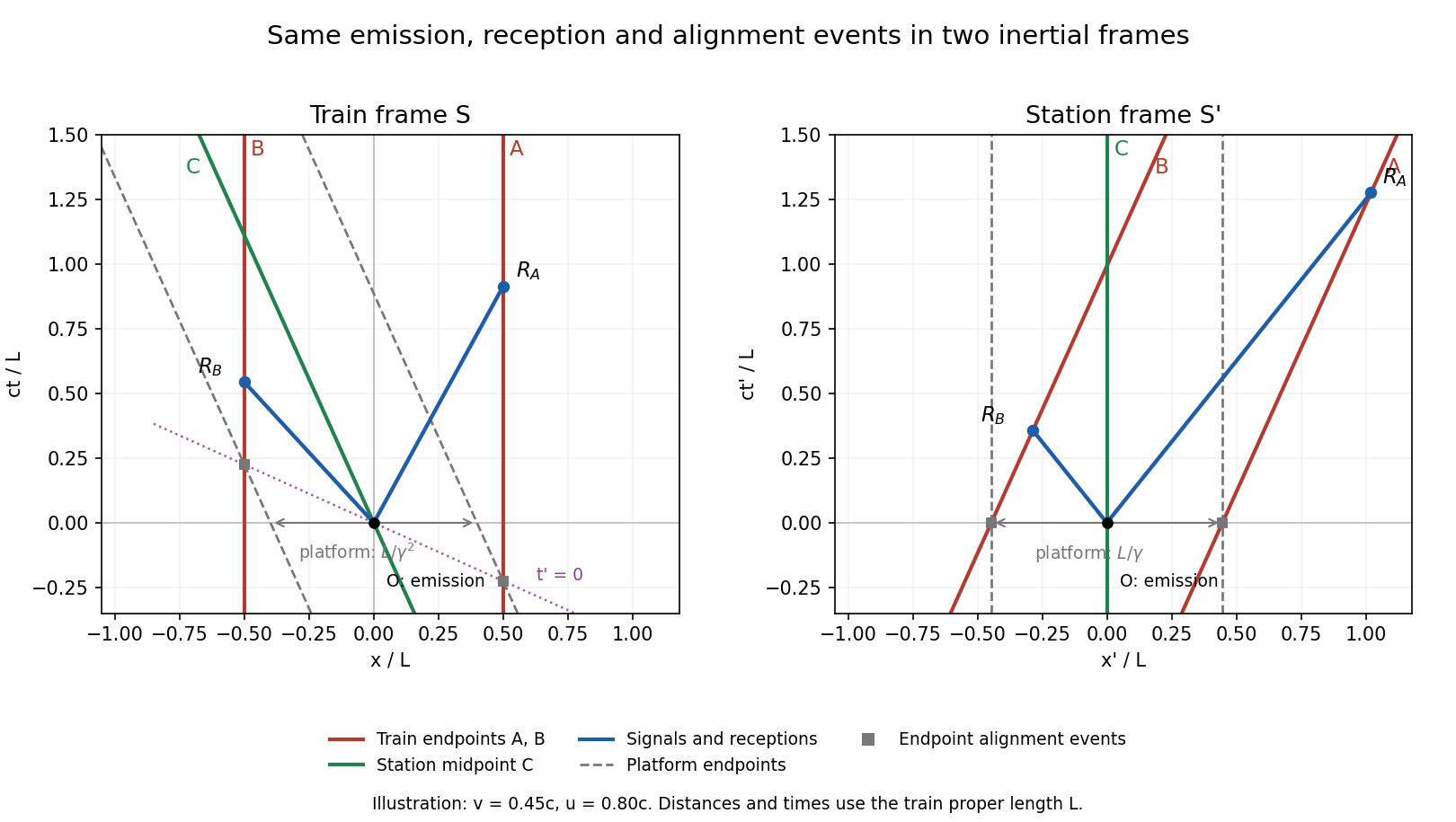

Let be the platform's proper length, measured in its rest frame . At the single station-frame time , its ends coincide with train endpoints whose simultaneous station-frame separation is . ThusThe platform endpoint world lines are vertical at in the station spacetime diagram. In the train frame they are , so their separation at a common train-frame time is . The two alignment events lie on the tilted line in the train diagram and are not simultaneous there; their separation cannot be used as the platform length measured at one train-frame time. This is the distinction enforced by length contraction.
In the station frame, intersecting the signal trajectories with the endpoint world lines givesSince , both receptions occur at positive times,The inverse Lorentz transformation then givesSubtracting and simplifying yieldsFor , both differences are negative: the rear receives first in both frames, but by different time intervals.
With light signals, , the train-frame relativistic velocity-addition formula gives signal velocities . The endpoints are equally distant from the source in that frame, andThe two reception events are simultaneous in but not in : in the station frame the rear moves toward its light signal while the front moves away. Directly, and , so the Lorentz transformation gives . This is relativity of simultaneity, concerning spatially separated events; it does not contradict the invariant light speed or the causal ordering of events on a single observer's world line.
For constant density , the inviscid Euler equations with conservative body force areThe vector identity simplifies for potential flow , since its vorticity vanishes. Also . ThereforeOn each connected fluid region the expression is spatially constant but may depend on time, giving the Unsteady Bernoulli equationThe arbitrariness of corresponds to the freedom to add a function of time to the velocity potential without changing . Replacing by sets the right-hand side to zero.
Use the ideal one-dimensional pipe model: constant density, steady inviscid flow, approximately uniform endpoint speeds , and equal body-force potential at the two ends. Conservation of mass gives the constant volumetric flow rate , and the mass flow rate is . The steady Bernoulli equation givesFor flow from a wider to a narrower section, and . Solving for the positive mass throughput gives the Venturi effect formulaThe formula requires these hydraulic assumptions; steady incompressibility alone does not impose uniform endpoint profiles or equal potential. If , the same derivation replaces by . Viscous losses would also modify the pressure balance. The equal-area case is singular in this pressure-based determination: in the ideal equal-potential model its pressure difference must vanish and does not determine the throughput.
Assume the explanatory variables are not all equal, so . In the Gaussian linear model, the log-likelihood isFor fixed , maximum likelihood estimation therefore minimizes the residual sum of squares. Differentiating in gives the least-squares normal equationsThe first gives ; substituting it into the second gives , with . Let . Differentiating the profiled log-likelihood in givesFor the variance estimator this is the interior maximum when , which occurs almost surely under the model when .
The coefficient estimators are linear functions of the independent normal errors. In particular,Their multivariate normal distribution has mean and covariance matrixThe fitted vector is the orthogonal projection onto the two-dimensional span of and . The residual vector is the complementary projection of the spherical normal error vector. Orthogonal normal projections are independent, and in an orthonormal basis of that complementary space its coordinates are independent . Consequentlyindependently of . This also gives the unbiased estimator rather than the variance MLE.
Under the null hypothesis , for the Student t test for a simple-regression intercept usesHere is the prescribed significance level. The normal numerator divided by its true standard deviation is independent of , which proves the stated Student t-distribution. If , the two coefficients are not separately identifiable; if , this residual-variance-based test is unavailable.
Set . The maximum likelihood estimation formulas for simple linear regression giveUsing the supplied rounded summaries gives metres and metres. Recomputing directly from the printed table gives approximately and metres, respectively, so the small summary rounding differences do not affect the conclusion.
I would not accept the model merely because the Student t-test fails to reject a zero regression intercept. That hypothesis test tests one parameter restriction within the assumed model, not the adequacy of its error assumptions or its functional form. In particular, complementary elevations and have exactly the same and hence the same fitted mean, but their observed low-angle minus high-angle ranges arefor the four corresponding pairs. All four are positive, suggesting an elevation-dependent effect omitted by the mean model, such as air resistance, rather than random scatter determined only by . This is a regression diagnostics concern, not a claim that these finite data logically rule out the normal-error model. The correct conclusion is nonrejection of the intercept restriction does not validate the regression model; further checks of the residual pattern and error assumptions are needed.
For fixed , put . Feasibility gives . The assumed Lagrangian duality representation says this value is the unrestricted supremum of , so is also an unconstrained global maximizer of this continuously differentiable function. Its first derivative vanishes:Differentiate the identity using the assumed smooth dependence of the optimizer:The chain rule now gives the envelope theoremThusEach Lagrange multiplier is the marginal change in optimal value per unit relaxation of its constraint. The proof only uses the resulting stationarity and smooth feasibility identities; it does not require differentiating the maximizer explicitly or differentiating the multiplier.
Capital and labour are nonnegative inputs. On the budget line, and . Both endpoints give zero output, whereas every interior point has positive output, so the maximum is interior. The Lagrangian with the sign convention of part (i) isIts stationarity equations are and . Dividing by the positive output gives and , hence . Together with the budget constraint this yieldsTo verify the unique global maximum, maximize the logarithm of the Cobb–Douglas production function along the budget line:Its unique stationary point is therefore the unique maximum, including comparison with the zero-output boundary points.
Writing and , the optimal output is . The Lagrange multiplier obtained from the first stationarity equation is . Direct differentiation verifies the envelope theorem identity:For clarity, the global dual-supremum premise of part (i) need not hold for every exponent pair allowed here. If , along the unrestricted Lagrangian is , which tends to infinity for every finite . Thus the verification above is by constrained stationarity and direct differentiation, and remains valid even when that stronger global Lagrangian duality representation fails.
Articles by others on the same topic
There are currently no matching articles.