Past exam of the mathematics course of the University of Cambridge / 2008 / ib

For $n\ge 1$, an eigenvalue is a number $\lambda \in \mathbb{C}$ for which there is a nonzero vector $v$ satisfying $Av=\lambda v$. Equivalently, $\ker (A-\lambda I)\ne \{0\}$, or $\det (A-\lambda I)=0$. The characteristic polynomial $\det (tI-A)$ has degree $n$ and leading coefficient one. By the fundamental theorem of algebra it has a complex root $\lambda$. At that root $A-\lambda I$ is a singular matrix, so it has a nonzero kernel vector, proving that $A$ has an eigenvalue.

True. If $Av=\lambda v$ with $v\ne 0$ and $A=A^{\ast }$, thenSince $v^{\ast }v>0$, $\lambda =\bar{\lambda }$. Thus every eigenvalue of a Hermitian matrix is real.

False. The matrix $A=\left(\begin{array}{cc}1& 1\\ 0& 2\end{array}\right)$ has real eigenvalues $1$ and $2$, because its characteristic polynomial is $(t-1)(t-2)$, but $A^{\ast }=\left(\begin{array}{cc}1& 0\\ 1& 2\end{array}\right)\ne A$. Real spectrum alone does not imply that it is a Hermitian matrix.

False. Every entry of $A=\left(\begin{array}{cc}1& 2\\ 2& 1\end{array}\right)$ is strictly positive, yet $A(1,-1{)}^T=-(1,-1{)}^T$. Its eigenvalues are $3$ and $-1$, so one has negative real part. Positivity of entries does not imply the positive-definite matrix property.

False in general. Take $A=\mathrm{diag}(1,6,6)$ and $B=\mathrm{diag}(2,2,9)$. Both have trace $13$ and determinant $36$, but their eigenvalue multisets are different. For $n>3$, append equal identity blocks to preserve this counterexample. In dimensions one and two the assertion is true: in dimension two the characteristic polynomial is $t^2-(\mathrm{tr}A)t+\det A$, whose roots, with multiplicity, are determined by those two quantities.

Let $Q\in \mathrm{SO}(3,\mathbb{R})$. Since $Q^{T}Q=I$ and $\det Q=1$,so $\det (Q-I)=0$. Choose a unit vector $e$ with $Qe=e$. Its orthogonal complement is an invariant subspace: for $v\perp e$, $e\cdot Qv=(Q^{T}e)\cdot v=e\cdot v=0$. In an orthonormal basis $(e,e_1,e_2)$, $Q$ therefore has a scalar block $1$ and a two-dimensional orthogonal matrix block of determinant one. Such a block has columns $(\cos \theta ,\sin \theta {)}^T$ and $(-\sin \theta ,\cos \theta {)}^T$. Consequently $Q$ is a rotation in three dimensions about the axis $\mathbb{R}e$ through angle $\theta$, including the identity when $\theta =0$.

To construct the Householder reflections, let $S_0$ reflect in the plane spanned by $e,e_1$ and let $S_{\psi }$ reflect in the plane spanned by $e,\cos \psi e_1+\sin \psi e_2$. They fix $e$, while on $e^{\perp }$ their matrices areTheir product is the planar rotation matrix through $2\psi$. Taking $\psi =\theta /2$ proves $\boxed{Q=S_{\theta /2}{S}_0}$. This gives the composition of two plane reflections explicitly; each is a Householder reflection $I-2n{n}^T$ for the corresponding unit plane normal $n$.

For a regular smooth curve $z=z_j(t)$ passing through $z_0$, the complex tangent of its image is $d{w}_j/dt=f^{\prime }(z_0)z_j^{\prime }(t)$. When $f^{\prime }(z_0)\ne 0$, both tangents are multiplied by the same nonzero complex number. Multiplication rescales lengths by $|f^{\prime }(z_0)|$ and rotates every direction by $\arg f^{\prime }(z_0)$, so the difference of tangent arguments is unchanged. Hence the analytic function defines a conformal map at $z_0$: oriented angles, and therefore ordinary angles between the curves, are preserved. The nonzero derivative condition also ensures that the image tangents are nonzero.

Write $f=u+iv$ and $z=x+iy$. The Cauchy-Riemann equations give $u_x=v_y$ and $u_y=-v_x$. Thus the real Jacobian determinant isThis identity also holds at points where $f^{\prime }(z)=0$; there the Jacobian is zero and local angle preservation is not guaranteed.

Choose the transverse axis so that the photon travels in the $xy$ plane. Its energy-momentum four-vector is $p^{\mu }=(E/c,E\cos \theta /c,E\sin \theta /c,0)$. A Lorentz boost of speed $v$ along $x$, with $\beta =v/c$ and $\gamma =(1-{\beta }^2{)}^{-1/2}$, givesBecause a photon has zero invariant mass, $|{\mathbf{p}}^{\prime }|=E^{\prime }/c$. ThereforeThe first is the relativistic Doppler effect in angular form, and the second is relativistic aberration.

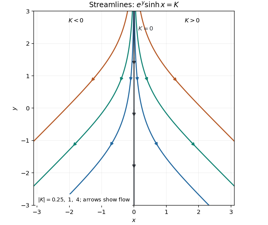
The divergence is ${\partial }_x(e^y\sinh x)+{\partial }_y(-e^y\cosh x)=e^y\cosh x-e^y\cosh x=0$, proving incompressibility. Use the stream function convention $u_x={\psi }_y$, $u_y=-{\psi }_x$. Integration of either component then givesThe streamlines are its level curves. Setting the irrelevant constant to zero, a nonzero level $K$ haswith $x>0$ for $K>0$ and $x<0$ for $K<0$. Each curve rises to $y=+\infty$ as $x\to 0$ from its side and approaches $y=\ln (2|K|)-|x|$ at large $|x|$. The zero streamline is $x=0$. Flow is downward everywhere, outward to the right when $x>0$ and outward to the left when $x<0$; on $x=0$ it is vertically downward.

A unit lower triangular $L$ is invertible. For $x\ne 0$, $y=L^{T}x\ne 0$, so an LDL decomposition with positive diagonal $D$ givesAlso $A=LD{L}^T$ is symmetric. Hence $A$ is a positive-definite matrix.

For the specified matrix, comparing entries successively gives $d_1=1$, $l_{21}=-1$, $l_{31}=2$, $d_2=3-l_{21}^2{d}_1=2$, andThusThe last pivot is negative, so this particular factorization is outside the positive-diagonal case proved above. Indeed $x=(-2,0,1{)}^T$ has $x^{T}Ax=-1$, and $\det A=-11$. There is no positive-diagonal LDL factorization for the printed matrix. The unrestricted LDL decomposition above is nevertheless valid.

Let $\bar{X}=n^{-1}{\sum }_i{X}_i$ and $S={\sum }_i(X_i-\bar{X}{)}^2$. The Gaussian distribution likelihood is proportional to ${\tau }^{n/2}\exp [-\tau {\sum }_i(X_i-\mu {)}^2/2]$. Multiplying by the normal-gamma distribution prior gives the quadratic exponent ${\sum }_i(X_i-\mu {)}^2+K_0(\mu -{\mu }_0{)}^2+2{\beta }_0$. Completing the square,The power of $\tau$ is ${\tau }^{{\alpha }_0+n/2-1}\sqrt{\tau }$, so the posterior distribution has exactly the required family withandFor a proper prior, $K_0,{\alpha }_0,{\beta }_0>0$ and ${\mu }_0\in \mathbb{R}$. The separate $\sqrt{\tau }$ factor is retained in both densities; it does not add $1/2$ to the update of $\alpha$. This is a conjugate prior for the Gaussian mean and precision parameter.

The Lagrangian sufficiency theorem for an equality constraint states that if a feasible $x_{\ast }$ and a multiplier ${\lambda }_{\ast }$ exist such that $x_{\ast }$ globally maximizes $L(x,{\lambda }_{\ast })=f(x)-{\lambda }_{\ast }\cdot (g(x)-b)$ over the underlying domain, then $x_{\ast }$ globally maximizes $f$ over $g(x)=b$. Indeed $L=f$ at every feasible point, so global maximality of $L$ directly compares the feasible objective values. The underlying domain can already impose $x_i\ge 0$.

For $0<p<1$, choose $\lambda =p{d}^{1-p}$. Each function $t^p-\lambda t$ on $t\ge 0$ is a strictly concave function and attains its unique maximum at $t=1/d$, since $p{t}^{p-1}=\lambda$ there. The sum Lagrangian is therefore globally maximized when every $x_i=1/d$, and this point is feasible. For $p=1$ the objective is identically one on the feasible set. For $p>1$, each feasible $x_i$ lies in $[0,1]$, so $x_i^p\le x_i$, with equality only at $0$ or $1$; equality in the total is attained exactly at a simplex vertex. ConsequentlyFor $0<p<1$ the unique maximizer is $(1/d,\dots ,1/d)$; for $p=1$ every feasible point is a maximizer; for $p>1$ the maximizers are exactly the $d$ vertices with one coordinate one and all others zero. When $d=1$ these descriptions coincide.

The row rank of $A$ is the dimension of the span of its rows in ${\mathbb{R}}^n$; its column rank is the dimension of the span of its columns in ${\mathbb{R}}^m$. Elementary row operations replace rows by invertible linear combinations, so preserve their span. They also preserve every column relation: $Ac=0$ if and only if $EAc=0$ for an invertible elementary matrix $E$. Reduce $A$ to row echelon form $R$, with $r$ nonzero rows. These rows are independent because their leading entries occur in distinct, successively later columns. The $r$ pivot columns are independent by their triangular pivot submatrix, while every column lies in the $r$-dimensional coordinate space supported on the nonzero rows. Thus both ranks of $R$, and hence both ranks of $A$, equal $r$. Row rank equals column rank.

Elementary column operations replace columns by invertible linear combinations and preserve their span. Equivalently, right multiplication by an invertible elementary matrix $F$ preserves row relations, since $c^{T}AF=0$ if and only if $c^{T}A=0$. Therefore either elementary row operations or elementary column operations preserve the matrix rank, and any finite sequence gives $\boxed{\mathrm{rank}(A^{\prime })=\mathrm{rank}(A)}$.

For the block matrices, put $M=\left(\begin{array}{cc}PQ& 0\\ Q& QR\end{array}\right)$. The explicit invertible multiplicationsfollow by first subtracting $P$ times the lower block row from the upper one and then subtracting the first block column times $R$ from the second. Changing the sign of the upper block row gives $N=\left(\begin{array}{cc}0& PQR\\ Q& 0\end{array}\right)$. These operations preserve matrix rank, proving that the two specified block matrices have equal rank. Their off-diagonal form gives $\mathrm{rank}(N)=\mathrm{rank}(Q)+\mathrm{rank}(PQR)$, since the two image components occupy independent coordinate blocks.

Choose $r_1=\mathrm{rank}(PQ)$ independent columns of $PQ$ and $r_2=\mathrm{rank}(QR)$ independent columns of $QR$. Select the corresponding $r_1$ columns from the first block column of $M$ and $r_2$ from the second. In a linear relation among these selected columns, the upper coordinate block forces every coefficient of the first selection to vanish; the lower block then forces every coefficient of the second to vanish. Consequently $\mathrm{rank}(M)\ge r_1+r_2$. Combining this with the equality of block ranks proves the Frobenius rank inequality:

The alternating group $A_4$ containsThe product of any two different nonidentity elements is the third, and each squares to the identity, so $V$ is a Klein four-group. Conjugation by a permutation replaces the labels in each cycle, preserving the property of being a product of two disjoint transpositions. Thus $V$ is a normal subgroup of $A_4$. Its order is $4$, strictly between $1$ and $|A_4|=12$. $A_4$ is not simple.

Write $G=\mathrm{Rot}(D)$ for the rotational symmetry group of a regular dodecahedron. Centre the solid at the origin. A rotation in three dimensions is determined by the image of a chosen face and one of its vertices, so there are at most $12\cdot 5=60$ rotations. All these choices occur. The outward unit normal to a face and the direction from its centre to the chosen vertex determine an oriented orthonormal frame. The proper rotation mapping one such frame to another maps the whole regular pentagonal face. At each edge, the common dihedral angle and convexity then determine the adjacent face uniquely; propagating across the connected face-adjacency graph shows that the rotation maps the entire solid to itself. Hence $|G|=60$, and the action is transitive on faces, vertices and edges.

Its rotations can be counted geometrically. There are six axes joining opposite face centres, each allowing four nonidentity rotations of order five; ten axes joining opposite vertices, each allowing two of order three; and fifteen axes joining opposite edge midpoints, each allowing a half-turn. The orbit-stabilizer theorem also verifies these possibilities: vertex stabilizers have order $60/20=3$ and edge stabilizers have order $60/30=2$, and their nonidentity elements rotate about the corresponding vertex or edge-midpoint axis. Together with the identity this accounts for all $1+24+20+15=60$ elements. In particular there are no elements of order four.

We now determine the conjugacy classes. The group is transitive on edges, so all fifteen edge half-turns are conjugate. For a rotation whose angle is neither zero nor $\pi$, a commuting rotation must preserve its oriented axis: conjugation carries the axis and its rotation angle to their images, and reversing the axis would reverse a non-half-turn angle. Thus its centralizer consists of rotations about the same axis. For a face rotation this centralizer has order five, and for a vertex rotation it has order three. The orbit-stabilizer theorem for conjugation therefore gives class sizes $60/5=12$ and $60/3=20$. The twenty vertex rotations form one class, and the twenty-four face rotations form two classes. The class sizes are $1,15,20,12,12$.

A normal subgroup is a union of these classes and contains the identity. Its possible orders areBy Lagrange's theorem its order must divide $60$. Only $1$ and $60$ in this list do so. Therefore $\boxed{G\text{ is simple of order }60}$.

For each involution $t\in G$, its conjugacy class has size fifteen, so its centralizer $C_G(t)$ has order four. A group of order four is a cyclic group or a Klein four-group; the cyclic possibility would contain an element of order four, excluded by the geometric enumeration. Hence each $C_G(t)$ is a Klein four-group containing three involutions.

If $u$ is any of the three involutions in $C_G(t)$, the latter group is an abelian group and hence is contained in $C_G(u)$. Both centralizers have order four, so they are equal. It follows that the fifteen involutions partition into five triples, with five distinct centralizers. Conjugation by $G$ permutes these five subgroups and gives a group homomorphism $\theta :G\to S_5$. This action is nontrivial: otherwise each of these order-four subgroups would be a normal subgroup, contrary to simplicity. The kernel of $\theta$ is normal; since $G$ is simple and the action nontrivial, its kernel is trivial. Thus $\theta$ is injective.

The sign of $\theta (g)$ defines a homomorphism $G\to \{\pm 1\}$. If it were nontrivial, simplicity would make it injective, impossible for a group of order sixty mapping into one of order two. Hence every image permutation is even, and $\theta (G)\subseteq A_5$. Both groups have order sixty, so they are equal. This constructs the requested group isomorphism:

The contraction mapping theorem states that a contraction mapping $T:X\to X$ on a nonempty complete metric space has a unique fixed point. Here contraction means that $d(Tx,Ty)\le qd(x,y)$ for all $x,y$, with one constant $0\le q<1$. Choose $x_0\in X$ and define $x_{n+1}=T{x}_n$. Successive distances satisfy $d(x_{n+1},x_n)\le q^{n}d(x_1,x_0)$, so for every $m\ge 1$,Thus $(x_n)$ is a Cauchy sequence. Completeness gives $x_n\to x_{\ast }$. Since a contraction mapping is a continuous function, $T{x}_{\ast }=\lim T{x}_n=\lim x_{n+1}=x_{\ast }$. If $y_{\ast }$ were another fixed point, $d(x_{\ast },y_{\ast })=d(T{x}_{\ast },T{y}_{\ast })\le qd(x_{\ast },y_{\ast })$, forcing distance zero. This proves both existence and uniqueness.

Now suppose $T=f^k$ is a contraction mapping, where $k$ is a positive integer. Let $y$ be its unique fixed point. Since $f$ commutes with its own iterate, $T(fy)=f(Ty)=fy$. Thus $fy$ is also a fixed point of $T$, so $fy=y$. Any fixed point of $f$ is a fixed point of $T$, and must equal $y$. A contractive iterate therefore gives a unique fixed point of $f$, without assuming continuity of $f$ itself.

The space $X=C([0,1],\mathbb{R})$ is complete for the uniform norm. Indeed, a uniformly Cauchy sequence converges pointwise by completeness of $\mathbb{R}$; passing to the limit in its uniform Cauchy bound shows uniform convergence, and the uniform limit of continuous functions is a continuous function. The operator $F$ maps this space to itself: $s\mapsto \varphi (h(s),s)$ is a continuous function, and its integral plus the continuous $g$ is a continuous function.

For $n=0$ the desired bound is the definition of $\Vert h-k{\Vert }_{\infty }$. Suppose it holds for $n$. The Lipschitz condition and the fact that the same $g$ cancels giveThis proves the estimate by induction. Taking the supremum over $0\le t\le 1$, the Lipschitz constant of $F^n$ is at most $M^n/n!$. These constants tend to zero, since the ratio of successive terms is $M/(n+1)$. Some iterate is consequently a contraction. The preceding result gives a unique fixed point of $F$, which is exactly $\boxed{\text{the unique continuous solution of the integral equation on }[0,1]}$. No assumption $M<1$ is needed.

A topology on $X$ is a family $\mathcal{T}$ of subsets containing $\varnothing$ and $X$, closed under arbitrary unions and finite intersections. Its members are the open sets. A Hausdorff space separates each pair of distinct points by disjoint open neighbourhoods; a compact space is one for which every open cover has a finite subcover.

Not a topology. Each singleton $\{n\}$ with $n>0$ is finite and hence belongs to the proposed family, but their union $\{1,2,3,\dots \}$ is infinite and excludes zero, so does not belong. The arbitrary-union axiom fails.

A Hausdorff compact topology. The empty set omits zero and $\mathbb{Z}$ has finite complement. An arbitrary union omitting zero belongs to the family. If a union contains zero, one of its constituent sets contains zero and is cofinite, so the union is also cofinite. A finite intersection either omits zero or is an intersection of finitely many cofinite sets and is therefore cofinite. This proves all topology axioms.

For distinct nonzero integers $a,b$, the disjoint open singletons $\{a\},\{b\}$ separate them. To separate $0$ and $n\ne 0$, use the disjoint open sets $\mathbb{Z}\setminus \{n\}$ and $\{n\}$. Thus this is a Hausdorff space. Every open cover has a member containing zero, which leaves only finitely many integers uncovered; choose one member for each of those points. This gives a finite subcover and proves compactness. The space is the one-point compactification of the discrete space $\mathbb{Z}\setminus \{0\}$, with zero as the added point.

Not a topology. For every integer $k\ge 2$, the set $U_k=\mathbb{Z}\setminus k\mathbb{Z}$ is periodic with period $k$, so belongs to the family. Their union is $\mathbb{Z}\setminus \{0\}$: for a nonzero $n$, choose $k>|n|$, which cannot divide $n$. But this union has no positive integer period. If it had period $k$, membership of $-k$ would force membership of zero. Again arbitrary unions fail the topology axiom.

A Hausdorff, noncompact topology. The condition says precisely that each point of $U$ lies in a residue class $n+k\mathbb{Z}$ contained in $U$. These classes form a basis: the intersection of two classes containing a common point contains the class through that point with modulus equal to the least common multiple of their moduli. Thus arbitrary unions obey the condition, and so do finite intersections. Also $\varnothing$ and $\mathbb{Z}$ obey it. This is the profinite topology on $\mathbb{Z}$.

If $a\ne b$, choose $k>|a-b|$. Then $a+k\mathbb{Z}$ and $b+k\mathbb{Z}$ are disjoint open neighbourhoods, proving the Hausdorff property. To test compactness, defineEvery $F_n$ is nonempty and both open and closed: its complement is a finite union of other residue classes. Since $a_{n+1}-a_n=4^n$, $F_{n+1}\subseteq F_n$. If $x$ belonged to their intersection, then $3x+1$ would be divisible by $4^n$ for every $n$, forcing $3x+1=0$, impossible for an integer. Therefore $U_n=\mathbb{Z}\setminus F_n$ is an increasing open cover of $\mathbb{Z}$. Any finite subcollection has union $U_N$ for its largest index and misses the nonempty $F_N$. This proves that the profinite topology on the integers is not compact.

Put $a=1/n$, so $0<a<1$, and write $I(a)={\int }_0^{\infty }{x}^a/(1+x^2)dx$. Choose the branch of the complex logarithm with $-\pi /2<\arg z<3\pi /2$, whose cut is the downward imaginary axis. Define $z^a=\exp (a\mathrm{Log}z)$ and integrate $z^a/(1+z^2)$ along the positively oriented upper semicircle, indented above zero. The straight pieces run from $-R$ to $-\epsilon$ and from $\epsilon$ to $R$; the small arc runs clockwise from argument $\pi$ to zero.

On the negative real axis $z^a=|z{|}^a{e}^{i\pi a}$, so the two straight pieces tend to $(1+e^{i\pi a})I(a)$. The outer arc is $O(R^{a-1})$ and the inner arc is $O({\epsilon }^{a+1})$, both tending to zero. The only enclosed pole is $i$, with residue $e^{i\pi a/2}/(2i)$. The residue theorem therefore givesUsing $1+e^{i\pi a}=2e^{i\pi a/2}\cos (\pi a/2)$ yieldsThe same bounds show convergence of the real integral at both zero and infinity.

Use the same indented upper-semicircle contour and branch of the complex logarithm, now for $F(z)=z^{1/2}\mathrm{Log}z/(1+z^2)$. Write $J={\int }_0^{\infty }{x}^{1/2}\log x/(1+x^2)dx$. On the negative axis, $z^{1/2}=i|z{|}^{1/2}$ and $\mathrm{Log}z=\log |z|+i\pi$. Consequently the two straight contributions tend toThe outer arc is $O(R^{-1/2}\log R)$ and the small arc is $O({\epsilon }^{3/2}(|\log \epsilon |+1))$, so neither contributes in the limit. At the enclosed pole $i$,The residue theorem gives $(1+i)J-\pi I(1/2)=i{\pi }^2{e}^{i\pi /4}/2$. Part (a) gives $I(1/2)=\pi /\sqrt{2}$. Substituting and using $e^{i\pi /4}=(1+i)/\sqrt{2}$, the right side after moving the $I$ term is ${\pi }^2(1+i)/(2\sqrt{2})$. Hence

For variations $y+ϵ\eta$ with $\eta (x_1)=\eta (x_2)=0$, integration by parts gives $\delta I={\int }_{x_1}^{x_2}[f_y-(d/dx)f_{y^{\prime }}]\eta dx$. Since this vanishes for every such variation, the Euler-Lagrange equation isWhen $f$ is independent of $y$, it has the first integral $\boxed{\partial f/\partial y^{\prime }=C}$.