Past exam of the mathematics course of the University of Cambridge / 2008 / ii / Paper 3

Put $N=\lfloor x\rfloor$. Comparing the harmonic number with an integral gives $H_N={\sum }_{n=1}^{N}1/n>{\int }_1^{N+1}dt/t=\log (N+1)>\log x$. By the fundamental theorem of arithmetic, the finite Euler product ${\prod }_{p\le x}(1-p^{-1}{)}^{-1}$ expands as the sum of $1/n$ over positive integers whose prime factors are at most $x$. It therefore includes every term of $H_N$, andThe first strict inequality is the geometric-series bound for the logarithmic remainder; the last uses the telescoping series ${\sum }_{n=2}^{\infty }1/[n(n-1)]=1$. Thus the prime reciprocal lower bound is

The closed-set version of the Baire category theorem says that if a nonempty complete metric space is a countable union of closed sets, at least one of those closed sets has nonempty interior. Equivalently, a nonempty complete metric space cannot be a countable union of closed nowhere dense sets.

Fix $ϵ>0$. For each $N$, the set $Q_N={\bigcap }_{n,m\ge N}\{x:|f_n(x)-f_m(x)|\le ϵ\}$ is closed, because each $f_n-f_m$ is continuous. At every $x$, pointwise convergence makes $(f_n(x))$ a Cauchy sequence, so $\mathbb{R}={\bigcup }_{N\ge 1}{Q}_N$. The Baire category theorem supplies an $N_0$ for which $Q_{N_0}$ contains a nonempty open interval $I$. For $x\in I$ and $n\ge N_0$, pass $m\to \infty$ in $|f_n(x)-f_m(x)|\le ϵ$ to obtainThis local uniform Cauchy control for pointwise convergent continuous functions allows both $I$ and $N_0$ to depend on $ϵ$.

Suppose a connected subset $C\subseteq F$ contains distinct points $a,b$. The distance function $d_a(x)=|x-a|$ is a Lipschitz map with constant one, by the reverse triangle inequality. Its image $d_a(C)$ is connected and contains both $0$ and $|b-a|$, so it contains the whole interval $[0,|b-a|]$. Monotonicity and the Lipschitz inequality for Hausdorff dimension implya contradiction. Thus every nonempty connected subset of $F$ is a single point: $F$ is totally disconnected. The argument is the Hausdorff dimension of a connected set bound, and does not require $F$ to be closed.

One choice of the Hamming code of length seven is the linear mapover ${\mathbb{F}}_2$. Its image is the kernel of the parity-check matrixIndeed $Hh(a,b,c,d{)}^T=0$, the encoder is injective because positions $3,5,6,7$ recover its inputs, and $H$ has rank three. Its columns are nonzero and pairwise distinct. Hence no nonzero codeword has Hamming weight one or two. The word $h(1,0,0,0)=(1,1,1,0,0,0,0)$ has weight three, proving that the minimum Hamming distance is three.

If $r=h(a,b,c,d)+e_j$ is received with one erroneous bit, its syndrome $H{r}^T$ is column $j$ of $H$. These seven columns are distinct, so the syndrome identifies the bit to flip. A zero syndrome indicates no error under the assumption of at most one error.

For the extended Hamming code, append ${\sum }_{j=1}^7{h}_j=a+b+c$. Every extended codeword has even weight. Since every original nonzero word has weight at least three, its extended weight is at least four; the weight-three example attains four. ThusThe minimum-distance error-detection and correction guarantee gives detection of up to three errors and correction of one error. Detection here means rejecting a word outside the code, rather than simultaneously identifying and correcting every detected pattern; the usual combined decoder corrects single errors and flags double errors.

The ordinary least squares estimate, which is also the maximum-likelihood estimate in this normal linear model, gives the hat matrixIt is the orthogonal projection onto the column space of $X$, so $P^T=P$, $P^2=P$ and $\mathrm{rank}P=p$. Since $(I-P)X=0$, the vector of regression residuals is $\widehat{ϵ}=(I-P)ϵ$, with multivariate normal distributionFor $i\ne j$, its covariance is $-{\sigma }^2{p}_{ij}$, which is generally nonzero. Therefore the regression residuals are generally dependent, even though the original errors are independent random variables.

Fit the model in R, compute its internally studentized residuals with rstandard(fit), and examine a normal Q-Q plot with qqnorm(rstandard(fit)) and qqline(rstandard(fit)). A plot of these regression residuals against the fitted values helps detect a curved mean pattern or nonconstant variance. Approximate agreement with a straight line in the Q-Q plot, with no systematic residual pattern, supports the assumed error model.

Here $p\ll n$. The average leverage is $\mathrm{tr}P/n=p/n$, and ${\sum }_{ij}{p}_{ij}^2=\mathrm{tr}(P^2)=p$. Thus most diagonal corrections and most off-diagonal dependences are small when only a few directions have been removed from a large sample. Also ${\tilde{\sigma }}^2$ estimates ${\sigma }^2$ accurately when $n-p$ is large. These facts make the visual independent-normal approximation reasonable, though exceptional high-leverage observations still deserve attention.

The approximation is not an exact distributional statement: the distribution of an internally studentized Gaussian residual has ${\hat{\eta }}_i^2/(n-p)\sim \mathrm{Beta}(1/2,(n-p-1)/2)$ when $n-p\ge 2$ and $p_{ii}<1$. In particular these residuals are bounded, rather than exactly distributed according to Student's t-distribution. Formal goodness-of-fit calibration should account for fitting and dependence.

Applying the law of mass action to the sequential two-site enzyme reaction network givesAdding the appropriate equations gives the conservation laws $e+c_1+c_2=e_0$ and $s+c_1+2c_2+p=s_0$. In particular $e=e_0(1-v_1-v_2)$ after nondimensionalization.

Define the dimensionless reaction rates $a_1=k_{-1}/(k_1{s}_0)$, $a_3=k_{-3}/(k_1{s}_0)$, $b_2=k_2/(k_1{s}_0)$, $b_4=k_4/(k_1{s}_0)$ and $r_3=k_3/k_1$. Substitution, with primes denoting $d/d\tau$, yieldsThese right sides are $f,g_1,g_2$, respectively, with $u(0)=1$ and $v_1(0)=v_2(0)=0$. When $ϵ\ll 1$, the form of these ordinary differential equations displays the faster relaxation of the complexes, which motivates a subsequent quasi-steady-state approximation.

The map normal forms at multiplier $+1$ are given in the numbered subparts below. For the multiplier $-1$ problem, the second iterate instead exposes the emerging period-two cycle.

For the multiplier $-1$ problem, write $x=X+\alpha /2$. To the required weighted order, with $X=O({\mu }^{1/2})$, the shifted map is $X_{n+1}=-X_n+b{X}_n+\gamma X_n^2+\delta X_n^3$, where $b=\beta +\alpha \gamma$. Composing it with itself cancels the quadratic term. The cubic contribution is $-2\delta X^3-2{\gamma }^2{X}^3$, while the linear correction is $-2bX$. Consequently the quadratic-cubic flip criticality calculation givesThus the second iterate has normal form $X_{n+2}=X_n+\hat{\mu }{X}_n-A{X}_n^3$, up to terms of weighted order at least four. This is the asymptotic interpretation of the stated remainder under $X=O({\mu }^{1/2})$; a uniformly valid local expansion about the exact fixed point also retains mixed parameter remainders.

Assuming $\hat{\mu }$ crosses zero transversely and $A\ne 0$, the small nonzero fixed points of the second iterate satisfy $X^2\sim \hat{\mu }/A$. They form a period-two orbit. For $A>0$ they exist on the side $\hat{\mu }>0$, where the original fixed point has become unstable, and the second-iterate multiplier is $1-2\hat{\mu }+o(\hat{\mu })$, so the cycle is stable. The period-doubling bifurcation is therefore supercritical precisely when $\delta +{\gamma }^2>0$. Equality is a degenerate case requiring higher-order terms.

A representative normal form for a saddle-node bifurcation of a map is $\boxed{x_{n+1}=x_n+\mu -x_n^2}$. Two fixed points $x=\pm \sqrt{\mu }$ appear for $\mu >0$; near the bifurcation the positive branch is stable and the negative branch unstable.

For a transcritical bifurcation, use $\boxed{x_{n+1}=x_n+\mu x_n-x_n^2}$. The fixed points $x=0$ and $x=\mu$ cross and exchange stability at $\mu =0$.

For a supercritical pitchfork bifurcation, use $\boxed{x_{n+1}=x_n+\mu x_n-x_n^3}$. The symmetric stable branches $x=\pm \sqrt{\mu }$ appear for $\mu >0$ as the origin becomes unstable. Replacing the cubic minus sign by plus gives a subcritical pitchfork bifurcation.

The Möbius transformation $w=z/(z-1)$ sends $0\mapsto 0$, $\infty \mapsto 1$ and $1\mapsto \infty$. The hypergeometric function $F(a,c-b;c;w)$ has local exponent pairs $(0,1-c)$ at $w=0$, $(0,b-a)$ at $w=1$, and $(a,c-b)$ at $w=\infty$. Pulling back to $z$ and multiplying by $(z-1{)}^{-a}$ gives the pairsAt infinity the prefactor adds $a$ to both exponents, while at $z=1$ it subtracts $a$ from both pulled-back exponents. These are exactly the requested Riemann P-symbol exponents. Equivalently, the Pfaff transformation identifies this branch, up to a nonzero phase depending on the chosen branches, with $F(a,b;c;z)$.

When $c\notin \mathbb{Z}$, an independent Frobenius solution isIts exponent $1-c$ differs from the first branch's exponent zero, establishing linear independence. For resonant parameters, use a parameter limit giving the appropriate logarithmic branch. More directly, on a simply connected region avoiding the singularities and zeros of a nonzero first solution $y_1$, reduction of order givesThe Wronskian is a nonzero multiple of $z^{-c}(1-z{)}^{c-a-b-1}$, so this also produces an independent local solution in the resonant cases for which the first branch is defined.

Let $A=Dy(x)$ be the Jacobian matrix and $K(y)=H(x(y))$. The chain rule gives ${\nabla }_{x}H=A^T{\nabla }_{y}K$. Therefore the Hamilton equations transform to $\dot{y}=AJ{A}^T{\nabla }_{y}K$, with $J=\left(\begin{array}{cc}0& -I\\ I& 0\end{array}\right)$. They have the required canonical form for every Hamiltonian exactly whenNecessity follows by choosing Hamiltonians whose gradients take arbitrary values at a point; sufficiency follows from the displayed transformed equation. This is the symplectic matrix condition for a canonical transformation, and it also forces $A$ to be invertible.

For the given transformation, $A=\left(\begin{array}{cc}1& 2\\ -1/4& 1/2\end{array}\right)$ has determinant one. For any $2\times 2$ matrix, $AJ{A}^T=(\det A)J$, so the proposed transformation is canonical.

Write the photon energy density as $ϵ=a_R{T}^4$, where $a_R=4\sigma /c$ by the Stefan–Boltzmann law. The photon gas has pressure $P=ϵ/3$ and zero photon chemical potential. The first law of thermodynamics therefore givesDividing by $T$ and integrating gives the entropy density of a photon gas:The integration constant is fixed to zero at zero temperature, consistently with the third law of thermodynamics.

The inequality $\Gamma \gg H$ says interactions act much faster than the expansion time, maintaining local thermal equilibrium. For adiabatic reversible expansion with no additional source of entropy, cosmological entropy conservation fixes the entropy in a comoving volume. Since that volume scales as $a^3$, and the relativistic degrees of freedom are fixed here, $T^3{a}^3$ is constant. ThusDuring radiation domination, the Friedmann equation gives $H^2\propto \rho \propto T^4$, and hence $\boxed{H\propto T^2}$. Fast interactions alone would not exclude an additional entropy-producing process; changing relativistic species likewise changes the simple temperature scaling.

For positive odd coprime integers $m,n$, the Jacobi reciprocity law isFactor $a={\prod }_j{q}_j^{e_j}$. Since $a$ is not a square, some $e_j$ is odd. Choose a quadratic nonresidue modulo that $q_j$, and choose residue one modulo each other $q_i$. The Chinese remainder theorem provides a positive $n$ with these residues and with $n\equiv 1(\mathrm{mod}4)$. Multiplicativity of the Jacobi symbol then gives $(n/a)=-1$.

Suppose only finitely many primes $p_1,\dots ,p_s$ satisfy $(a/p_i)=-1$. They are coprime to $a$. Repeat the preceding Chinese remainder theorem construction, additionally imposing $n\equiv 1(\mathrm{mod}{p}_i)$ at every odd $p_i$ and taking $n\equiv 1(\mathrm{mod}4)$ to avoid two. Since $n\equiv 1(\mathrm{mod}4)$, Jacobi reciprocity gives $(a/n)=(n/a)=-1$. Factoring this Jacobi symbol over the prime factors of $n$ shows that at least one such prime $p$ has $(a/p)=-1$. But none of the listed primes divides $n$, a contradiction. This proves the infinitely many prime quadratic nonresidues of a nonsquare integer assertion.

The Liouville approximation theorem says that for a real algebraic number $\xi$ of degree $d\ge 2$, there is a constant $C(\xi )>0$ such thatfor all integers $p$ and $q\ge 1$ with $p/q\ne \xi$. In particular a quadratic irrational cannot have arbitrarily accurate rational approximations of order $o(q^{-2})$.

The matrix recurrence gives $p_{n+1}{q}_n-p_n{q}_{n+1}=(-1{)}^n$ and $q_{n+1}=a_{n+1}{q}_n+q_{n-1}$. Successive continued fraction convergents bracket $x$, henceThe infinite continued fraction is irrational: if $x=p/q$ were rational, a distinct convergent would be at distance at least $1/(q{q}_n)$, contradicting the first bound once $q_{n+1}>q$. If $x^2$ were rational, this irrational $x$ would have degree two. The Liouville approximation theorem would then give $|x-p_n/q_n|\ge C/q_n^2$. Comparing with the displayed bound would force $a_{n+1}\le 1/C$ for every $n$, contrary to the unbounded coefficients. Thus $x^2$ is irrational, by the unbounded continued-fraction coefficients exclude quadratic irrationality argument.

For a small Fourier mode $u=U{e}^{ikx+\sigma t}$, $v=V{e}^{ikx+\sigma t}$, the inhibitor equation gives $V=U/(1+k^2)$. The linearization of the cubic reaction at zero is $-rU$. Thus the fast-inhibitor cubic activator growth rate isIt is an even function of $k$, starts at $\sigma (0)=-r<0$, and tends to $-\infty$ as $|k|\to \infty$. In terms of $q=k^2$, its derivative is $-D+\rho /(1+q{)}^2$. If $\rho >D$, the maxima occur at $k=\pm \sqrt{\sqrt{\rho /D}-1}$, withIf $\rho \le D$, the maximum is $-r$ at $k=0$ and all modes decay. For $\rho >D$, the zero state is unstable when $(\sqrt{\rho }-\sqrt{D}{)}^2>r$, and the stability boundary iswhere this curve lies in the allowed parameter region.

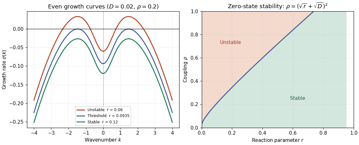
Putting $\tilde{u}=1-u$, $\tilde{v}=1-v$ and $\tilde{r}=1-r$ negates both original equations and restores precisely the same form, because $\tilde{u}(\tilde{u}-\tilde{r})(\tilde{u}-1)=-u(u-r)(u-1)$. Therefore the state $u=v=1$ has the corresponding boundary $\boxed{\rho =(\sqrt{1-r}+\sqrt{D}{)}^2}$.

For a positively oriented simple closed curve on which the vector field is nonzero, its Poincaré index is the total rotation of the vector field along that curve divided by $2\pi$, equivalently the winding number of its normalized direction. The Poincaré index of an isolated fixed point is that of a sufficiently small enclosing curve containing no other fixed point. The index of a planar periodic orbit is $+1$.

The equilibrium points are $(0,0)$ and $(\pm 1,\pm (b-a))$, with correlated signs. The Jacobian matrix is $\left(\begin{array}{cc}a-3b{x}^2& 1\\ 3x^2-1& 0\end{array}\right)$. At the origin its eigenvalues satisfy ${\lambda }^2-a\lambda +1=0$. It is a focus for $0<|a|<2$, a repeated-eigenvalue node for $|a|=2$, and a node for $|a|>2$; stability is determined by the sign of $a$, with stability for $a<0$. Its Poincaré index is $+1$. At either other equilibrium the determinant is $-2$, so it is a saddle point with Poincaré index $-1$.

Take $H(x,y)=y^2/2+x^2/2-x^4/4$. Along a trajectory,Integrating over a periodic orbit returns $H$ to its starting value, and henceThis is the energy obstruction for a cubic planar oscillator.

The second-order equation is equivalent to the planar system after setting $y=\dot{x}-ax+b{x}^3$. Any nonconstant periodic solution has a maximum $M$ and minimum $m$. At an extremum $\ddot{x}=x^3-x$, so $M>1$ and $m<-1$ are impossible. Equality at either endpoint would give one of the equilibrium points, and uniqueness would force a constant solution. Therefore a nonconstant periodic orbit lies in $-1<x<1$.

If $b/a<1$, throughout this striphas the sign of $a$ whenever $x\ne 0$. A nonconstant orbit spends a positive time away from $x=0$, so its integral cannot vanish, contradicting part (b). Thus there are no nonconstant periodic solutions. The constant equilibrium solutions of course remain; as usual the question's periodic-orbit assertion excludes equilibria.

In a flat matter-dominated universe, $a\propto t^{2/3}$, $H=2/(3t)$ and $4\pi G{\bar{\rho }}_c=2/(3t^2)$. Substitution of ${\delta }_k\propto t^{\beta }$ gives $\beta (\beta -1)+(4/3)\beta -2/3=0$, whose roots are $2/3$ and $-1$. HenceDuring radiation domination, $a\propto t^{1/2}$ while ${\bar{\rho }}_c/{\bar{\rho }}_{\mathrm{total}}\propto a\ll 1$. The matter self-gravity term is suppressed relative to $H^2$, leaving approximately ${\ddot{\delta }}_k+t^{-1}{\dot{\delta }}_k=0$, with solutions constant and $\log t$. Thus there is no growing power-law mode comparable to the later $t^{2/3}$ growth. The elementary estimate in part (ii) neglects this slow logarithmic growth of matter perturbations during radiation domination.

Normalize $a(t_0)=1$. In the matter era, horizon crossing $c{t}_H=2\pi a(t_H)/k$ with $a=(t/t_0{)}^{2/3}$ gives $t_H/t_0=(k_0/k{)}^3$. In the radiation era, match $a=(t_{\mathrm{eq}}/t_0{)}^{2/3}(t/t_{\mathrm{eq}}{)}^{1/2}$ to obtainThe boundary mode therefore has $k_{\mathrm{eq}}=k_0(1+z_{\mathrm{eq}}{)}^{1/2}$. For $k<k_{\mathrm{eq}}$, the growing mode multiplies the primordial amplitude by $(t_0/t_H{)}^{2/3}=(k/k_0{)}^2$. For $k>k_{\mathrm{eq}}$, growth is approximately frozen until equality, then multiplied by $(t_0/t_{\mathrm{eq}}{)}^{2/3}=1+z_{\mathrm{eq}}=(k_{\mathrm{eq}}/k_0{)}^2$. Squaring these factors gives the matter power spectrumThe large-$k$ estimate omits the logarithmic radiation-era transfer correction, consistently with the stipulated approximation.

A transitive set $x$ satisfies $z\in y\in x\Rightarrow z\in x$, equivalently $\bigcup x\subseteq x$. If $x$ is transitive and $z\in y\in \bigcup x$, choose $w\in x$ with $y\in w$. Transitivity gives $y\in x$, so $z\in \bigcup x$. Thus $\bigcup x$ is transitive. If $z\in y\in \mathcal{P}(x)$, then $z\in x$ and transitivity implies $z\subseteq x$, whence $z\in \mathcal{P}(x)$. Thus the power set is transitive as well.

The converse for the union is false: take $x=\{\{\varnothing \}\}$. Then $\bigcup x=\{\varnothing \}$ is transitive but $x$ is not. The power-set converse is true: if $z\in y\in x$, then $y\in \{y\}\in \mathcal{P}(x)$ implies $y\in \mathcal{P}(x)$, so $z\in x$.

Define $x_0=x$, $x_{n+1}=\bigcup x_n$ and $\mathrm{TC}(x)={\bigcup }_{n<\omega }{x}_n$. This is a set by replacement and union, contains $x$ as a subset, and is transitive because taking a member advances one stage. Induction shows it is contained in every transitive set containing $x$, proving the transitive closure property.

If the rank of a set $x$ is $\alpha$, thenEvery subset of $x$ has rank at most $\alpha$, and $x$ itself is an element of $\mathcal{P}(x)$, proving the first formula. The second is transitive closure preserves set-theoretic rank. Here the convention is $x\subseteq \mathrm{TC}(x)$, not $x\in \mathrm{TC}(x)$.

The chromatic polynomial $p_G(t)$ counts proper vertex colorings with $t$ labeled colors at positive integer $t$. For an edge $e$, the deletion-contraction recurrence for the chromatic polynomial is $p_G=p_{G-e}-p_{G/e}$, where parallel edges in the contracted graph are merged. Induction on edges, starting from the edgeless polynomial $t^n$, shows that the coefficients have alternating signs: the contracted graph has one fewer vertex, so subtracting its alternating polynomial reinforces the same signs. The leading coefficient stays one. The coefficient of $t^{n-1}$ decreases by one per added edge, hence it is $-m$. Thus $p_G(t)={\sum }_{i=0}^n(-1{)}^{n-i}{a}_i{t}^i$, with $a_n=1$, $a_{n-1}=m$ and all $a_i\ge 0$.

For a tree, choose a root, give it any of $t$ colors, and give every other vertex any of the $t-1$ colors different from its parent. This gives $p_G(t)=t(t-1{)}^{n-1}$. Conversely, a graph with this polynomial has $m=n-1$. The chromatic polynomial of a disjoint union is the product of those of its connected components, each divisible by $t$. The given polynomial has a simple zero at zero, forcing a single connected component. A connected graph with $n-1$ edges is a tree. The converse holds.

Finally the polynomial determines the number of vertices, the number of edges and the chromatic number. If it equals that of the Turán graph $T_r(n)$, with $1\le r\le n$, then $G$ has chromatic number $r$, so has no $K_{r+1}$, and has the maximum possible number of edges for such a graph. The equality case in Turán's theorem makes $G$ isomorphic to $T_r(n)$. This is the chromatic polynomial determines a Turán graph property. If $r>n$, the graph is simply complete and its edge count already determines it.

An algebraic element $\alpha$ over $K$ is a root of a nonzero polynomial in $K[T]$. Its degree is the degree of its minimal polynomial, equivalently $[K(\alpha ):K]$. Since $\alpha$ satisfies $T^2-{\alpha }^2$ over $K({\alpha }^2)$, the tower law gives $[K(\alpha ):K({\alpha }^2)]\le 2$ and makes that degree divide the odd integer $[K(\alpha ):K]$. It must therefore be one, proving $\boxed{K(\alpha )=K({\alpha }^2)}$.

For the addition assertion, let polynomial relations of degrees $r,s$ express ${\alpha }^r$ and ${\beta }^s$ in terms of lower powers. The finite-dimensional $K$-space spanned by ${\alpha }^i{\beta }^j$ for $0\le i<r$, $0\le j<s$ contains one and is closed under multiplication by $\alpha +\beta$. Thus $1,\alpha +\beta ,\dots ,(\alpha +\beta {)}^{rs}$ are linearly dependent. Their dependence is a nonzero polynomial relation over $K$, so $\alpha +\beta$ is algebraic.

A separable algebraic element has a minimal polynomial with distinct roots in an algebraic closure. A separable field extension is an algebraic extension all of whose elements are separable. In characteristic $p$, the extension ${\mathbb{F}}_p(t)/{\mathbb{F}}_p(t^p)$ is inseparable: the minimal polynomial of $t$ is $T^p-t^p$, irreducible over the smaller field but having the single root $t$ with multiplicity $p$.

If $L$ is a finite field of order $q$, every element of $L$ is a root of $T^q-T\in K[T]$, because $K$ contains its prime field. This polynomial has derivative $-1$, so it has no repeated roots. Every element's minimal polynomial divides it and is therefore separable. Hence $L/K$ is separable.

On a maximal torus element $\mathrm{diag}(t,t^{-1})$, the SU(2) representation $V_2$ has weights $2,0,-2$. A monomial with respective multiplicities $a,b,c$ has weight $2(a-c)$, givingFor $0\le \ell \le n$, its weight-$2\ell$ multiplicity is $\lfloor (n-\ell )/2\rfloor +1$, and multiplicities are symmetric in $\ell$. An irreducible $V_{2j}$ contributes one at each weight $2j,2j-2,\dots ,-2j$, so subtracting adjacent multiplicities yields the symmetric powers of the three-dimensional SU2 representation decompositionIt contains the trivial representation once when $n$ is even, and never when $n$ is odd. ThereforeThe double cover $SU(2)\to SO(3)$ identifies $V_2$ with the complexified standard three-dimensional representation. It is self-dual, so the same invariant dimensions apply to homogeneous polynomials. The quadratic form $q=x^2+y^2+z^2$ is invariant, and its powers give nonzero invariants in every even degree. Since each such degree has dimension one and each odd degree has dimension zero, every invariant is a polynomial in $q$. There is no polynomial relation on $q$, as seen by setting $y=z=0$. Thus