For a real number , set and . If , define . The resulting simple continued fraction is , where is an integer and subsequent are positive integers. It terminates when a complete quotient is integral; otherwise its convergents tend to .
For the continued fraction of the square root of nineteen, the complete quotients after areTheir integer parts are . Taking the reciprocal after subtracting from the last quotient returns the first one, so
The nonzero leading coefficients and distinct degrees make a basis of the polynomials of degree at most . Consequently the given orthogonality implies for every such polynomial .
If has infinitely many distinct zeros in , there is nothing to prove. Otherwise suppose it has fewer than . Among those zeros, list the sign-changing ones as , with , and put , using when . On each interval between zeros, has a fixed sign by continuity. Crossing a sign-changing zero flips both and ; crossing any other zero flips neither sign. Thus has one constant sign wherever nonzero. Since is not identically zero, continuity gives an open interval on which is strictly of that sign. Hence its integral is nonzero, contrary to orthogonality to . Therefore has at least distinct zeros in . This is the reusable orthogonality forces many interior zeros argument.
Let be an isometry, and set . Then , and preservation of distances gives . The polarization identity yieldsFor a standard orthonormal basis , put . These three vectors are an orthonormal basis. Since , we have for an orthogonal matrix . Thusan affine map.
For a finite isometry group , take . An affine map preserves an affine average, so for any ,The orbit barycentre is a common fixed point. This proves the fixed point of a finite Euclidean isometry group result.
If the possible values have probabilities , allowing zeros, the Shannon entropy in bits is , with . Each term is nonnegative, so , with equality precisely when one value has probability one.
For the upper bound, prove first that for : the function has derivative and its unique minimum, zero, at . Let be the number of positive probabilities. Applying this inequality to givesThe left side is , provingEquality at the maximum requires and equality in every logarithmic inequality, so every . Conversely the uniform distribution attains it. For the maximum and minimum coincide at zero.
The inverse logit link is . independence therefore gives the Likelihood function and log-likelihoodDifferentiation yields the score . The matrix whose rows are has dimension , not the PDF's printed . With this necessary dimension correction, any finite maximum Likelihood function estimate satisfiesThe Hessian matrix is , with , so the log-likelihood is concave. These score equations apply to a finite interior estimate; complete or quasi-complete separation can instead make its supremum occur only as coefficients diverge.
The deviance is twice the difference between maximized saturated and fitted log-likelihoods. A saturated Bernoulli distribution has fitted means and log-likelihood zero, interpreted by limits. Hence the binomial deviance here isZero-multiplier logarithms are interpreted as zero.
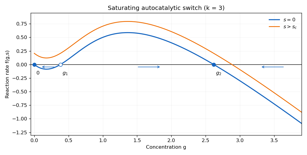
Continue in the bistable regime . At the reaction function factors as . Besides , its positive equilibria areAt zero, , so it is stable. At a positive equilibrium, use to obtain . Therefore is unstable and stable. The sign of is negative on , positive on and negative beyond ; these signs determine the requested reaction-rate sketch.
The stationary points of obey . For its smaller solution is the local minimum, and its larger solution lies above one and is the local maximum. Since increasing translates the whole graph upward, the low and middle equilibria collide whenFor , both stationary values of are positive, while as ; there is exactly one nonnegative equilibrium, on the descending high branch. At equality a double low equilibrium remains, so the uniqueness assertion requires strict exceedance.
For completeness, if the later positive-input request is considered for arbitrary , the derivative is . Its maximum is , attained at . For , the reaction graph is decreasing and every already has a unique steady state, so take . For , the smaller positive stationary point gives the same ; above it the graph crosses zero only on its final descending branch. Persistent robust switching after input is removed uses the previously assumed bistable regime .
Starting near zero, raise past and keep it there long enough for to pass the unstable threshold and approach the high branch. Decrease back to zero slowly, or after ensuring . The trajectory then stays in the basin of the high stable equilibrium and ends at the displayed . The persistent switched state is . This is the saturating autocatalytic switch; the conclusion presupposes and enough forcing duration, not merely an arbitrarily short pulse of large amplitude.

For , the first integralhas . The equilibrium points are and . The linearization has eigenvalues at the origin and at . The origin is a center equilibrium: the sufficiently small positive level sets of are closed curves, since its Hessian matrix there is positive-definite. The other equilibrium is a saddle equilibrium.
At the saddle, , and the separatrix satisfiesIts two branches with form a homoclinic orbit through the saddle; its remaining branches extend to . Inside the loop, the closed trajectories run clockwise: above the horizontal axis . The saddle directions have slopes and . Outside the loop there are unbounded trajectories. The left panel shows the closed orbits and all saddle branches.
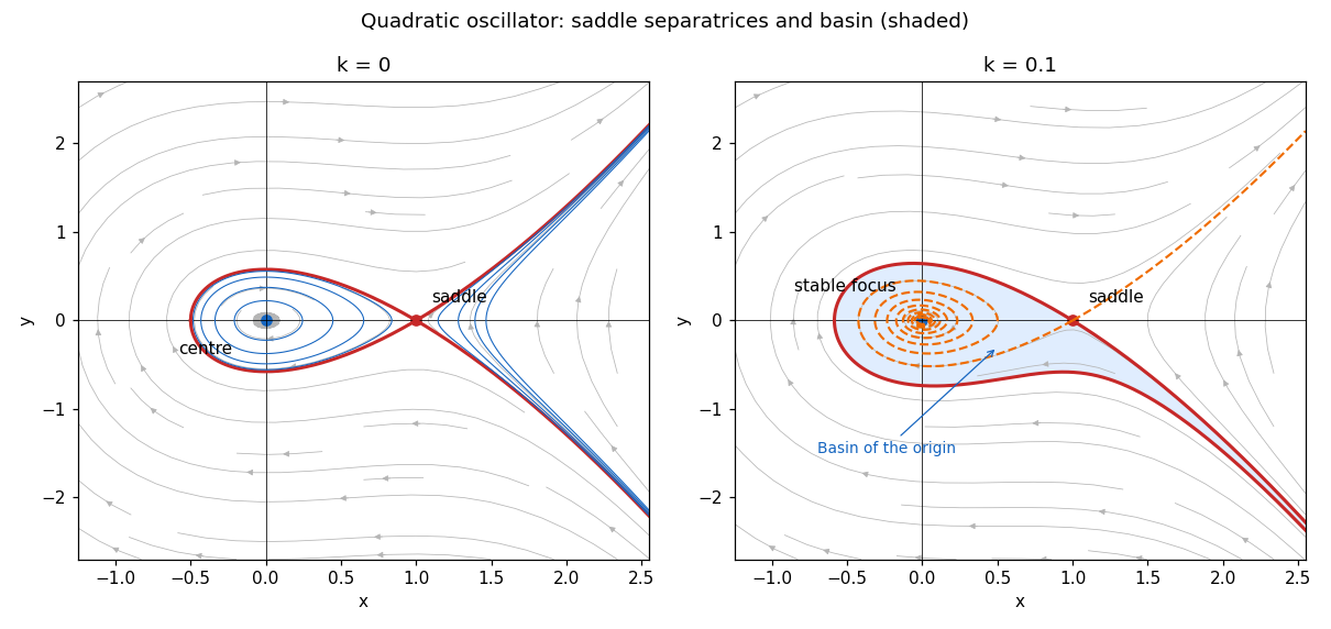
Conservative phase portrait and the attracting basin after adding weak damping
. Details. 
For general , the same energy gives . For the eigenvalues at the origin are , so it is a stable focus. At they are , so it remains a saddle equilibrium. The vector field has constant divergence : there are no periodic orbits, by the planar divergence criterion. Nor can the former homoclinic orbit survive, since strictly decreases along every nonconstant orbit except at isolated crossings of .
The stable manifold of the saddle separates escape to positive from convergence to the origin. Its two branches approach the saddle in forward time with tangent slope . The left unstable branch spirals into the origin, whereas the right unstable branch escapes. The shaded component on the origin's side of the stable manifold in the right panel is the basin of attraction. The boundary itself is excluded: its trajectories converge to the saddle. This boundary is the damped stable manifold, rather than the conservative energy contour. energy decrease prevents bounded recurrent motion, and every bounded orbit off the saddle's stable manifold consequently converges to the origin. The plotted manifold was obtained by integrating backwards from the saddle's stable eigendirection.
Near zero the magnitude of the integrand is of order , and at infinity it is of order . Thus the improper integral converges exactly in the stripAt a boundary of this strip the logarithmic-variable oscillation has no limiting primitive, so conditional convergence does not enlarge it.
Use a keyhole contour about the positive real axis for , taking . The circular arcs vanish in the indicated strip. The upper and lower banks contribute . The only enclosed pole is the double pole at , whose residue is . The residue theorem therefore givesAt the quotient has a removable singularity, with limit one, agreeing with .
For an arbitrary smooth variation vanishing at both endpoints,The endpoint term in integration by parts is zero. stationarity for every variation and the fundamental lemma of the calculus of variations imply the Euler-Lagrange equations . Least action here means stationary action, not necessarily a global minimum. The conjugate momentum is ; a cyclic coordinate, , makes constant.
For the symmetric top, and are cyclic. Thusare constant, and consequently so is . Conservation of energy from time-translation invariance also supplies the conserved energyThese give the requested additional conserved quantities and . The equation isFor constant and constant precession rate , it reduces toConversely, choose constants satisfying this balance and set . The cyclic equations and equation are then all satisfied, so this constructs uniform precession wherever the Euler-angle chart is regular.
In the nonrelativistic dilute regime, and , so the Bose or Fermi correction in the denominator is negligible. The common Maxwell-Boltzmann distribution approximation givesDifferentiating the quoted Gaussian integral with respect to its squared scale gives . Thereforechemical equilibrium of requires . Apply the density formula to each species to obtainUsing , the specified , and , , givesFor and , the corresponding deuterium equilibrium abundance isThe very small baryon-to-photon ratio means that even the high-energy tail contains many photons per baryon capable of destroying deuterium when is of order . Substantial deuterium survives only after that tail has been exponentially suppressed, so must be large enough to offset the small prefactor. This is the deuterium bottleneck, not a threshold set just by equality of thermal energy and binding energy. The degeneracy is used as stipulated for this calculation.
inversion in a circle with center and radius is , with and infinity interchanged. It fixes the circle pointwise and reverses complex orientation. Each inversion is fractional-linear in , so composing two eliminates the conjugation and gives with nonzero determinant: a Möbius transformation.
Translate and rotate two distinct centers to , where , and let the radii be . The composition of inversion in the first circle followed by the second isIts fixed points solve . The discriminant isDisjoint circle boundaries require either or , so both factors have the same nonzero sign and . There are two distinct fixed points on the line of centers. If the circles are concentric, their radii differ and the composition is , with exactly the two fixed points . Thus the composition has two distinct fixed points, also for nested disjoint circles. Reversing the order inverts the Möbius transformation and leaves its fixed points unchanged.
For a binary symmetric channel with crossover probability , Shannon's noisy coding theorem gives capacity bits per use, where . For any rate below capacity there are block codes with block length tending to infinity and decoding error tending to zero. Conversely, vanishing-error transmission cannot have asymptotic rate above capacity. At the capacity is zero; the formula also covers by complementing the output.
For discrete random variables, mutual information isThe formula is symmetric. To prove nonnegativity, apply to for positive joint masses. Multiplication by and summation gives . Hence , with equality precisely for independence. The channel information capacity is , over input distributions.
For the ternary channel every conditional output row has entropy , independent of the input. Therefore . Uniform input produces uniform output, since the matrix is doubly stochastic, and attains the bound. ThusUse at the endpoints. At the noiseless capacity is ; at all output rows are uniform and capacity is zero.
The array has replicates, levels of factor , and levels of factor , giving . R vectorizes an array with the first index changing fastest, then the second, then the third. Accordingly,
gl(I,K,length(y)) repeats each level for the ten replicates and cycles over its two levels, while gl(J,K*I,length(y)) repeats each level for twenty observations. These factors align with the vectorized response.The first fit is the additive Analysis of variance model , with independent normal errors of common variance . Under the default treatment constraints , the four fitted coefficients estimate the baseline cell mean, the minus effect, and the contrasts with . Thus the baseline fitted mean is , the second level adds , and the second and third levels add and .
The summary tests compare each indicated coefficient with zero, using its standard error and residual variance estimate . They have 56 residual degrees of freedom. The three non-intercept contrasts are strongly significant; the intercept test asks whether the baseline mean is zero, not whether either factor matters overall. The Analysis of variance tests are joint nested-model tests: no main effect, with one numerator degree of freedom, and no main effect, with two. Their sequential sums of squares are and . In this balanced design the main-effect subspaces are orthogonal, so ordering does not change those sums of squares. The denominator is the same residual mean square ; both factor effects are highly significant.
The second fit expands
a*b to a+b+a:b, adding two interaction coefficients. It allows the effect to differ between levels and has six parameters, equivalently one mean per cell, with 54 residual degrees of freedom. The interaction adds only about to explained sum of squares; its statistic is with degrees of freedom and . There is no evidence against additivity, so the simpler first model is preferable on these data. This does not prove the true interaction is exactly zero.For the final expression, , , and . The fitted vectors are orthogonal projections onto nested model spaces, so is the additional sum of squares due to interaction. The final code computesthe same interaction test as the Analysis of variance row. The exact value uses the original, unrounded observations and fits. Using only the displayed rounded sums and gives about instead; that discrepancy is rounding, not a different test. The omitted observations prevent reconstructing more digits from the printed data alone.
The chain rule gives , , and . Thereforewhich, after division, is the printed equation. It has only three regular singular points, , and is thus a Papperitz equation. At zero and one the indicial roots are . At infinity, inserting gives . Its Papperitz symbol isThe exponent sum is one, as required for a three-singularity second-order equation.
Multiplying the equation by puts it in Gauss hypergeometric equation form with , , . The solution analytic at zero and normalized to one is . Composing it with gives an even analytic solution of with , . Uniqueness of this ordinary differential equation impliesThis Gauss hypergeometric function identity initially holds near zero, and on with the usual real branch; it extends by matching analytic continuation. It is not an identity on every real if the left side is always reevaluated on its principal branch: for that principal value is . Continuing the branch consistently restores the stated cosine.
Let a comoving test particle have physical radius , where is fixed. Assume Newtonian gravity, spherical homogeneity, negligible pressure, and no mass flux through this sphere, so its enclosed mass is constant. The shell theorem gives a conserved specific energySubstitute , divide by , and write to obtainHomogeneity makes the energy scale as , leaving the same at every comoving radius. The sign of encodes the binding-energy sign. This Newtonian derivation applies to pressure-free matter; interpreting as spatial curvature and extending the equation to relativistic pressure components requires general relativity, rather than conservation of this Newtonian shell energy alone.
Separate fluid conservation gives , hence after normalization at today. For , the conservation equation gives . ThusAssume both densities are positive and set , . On the expanding flat branch, . With this becomes . Choosing the Big Bang at and integrating givesThe normalization requires ; equivalently . Thus the age and the two positive densities are not independent once this normalization and bang time are fixed.
As , , the matter-dominated law. As , and , giving accelerated dark-energy expansion. Direct differentiation gives , so acceleration begins once . If dark energy vanishes, the limiting matter-only solution must be taken instead; negative dark-energy density would not have the stated late-time accelerating form.
A well-order is a linearly ordered set in which every nonempty subset has a least element. First note that a well-order cannot be isomorphic to a proper initial segment of itself: the least element moved by such an isomorphism would have exactly the same predecessor set on each side, forcing it to be fixed. The same least-disagreement argument makes an isomorphism between initial segments unique.
Match to exactly when their strict predecessor sets are order-isomorphic. The preceding observation makes each match unique. Matches preserve order and fill initial segments on both sides, since restricting an isomorphism matches every earlier element. If both sides had an unmatched element, take the least unmatched and . Their predecessor sets would be exactly the already matched segments, so they too would match, a contradiction. Therefore the matching exhausts at least one well-order and gives an isomorphism of that whole set onto an initial segment of the other. Uniqueness follows from the same predecessor-set argument. The whole set is allowed as an initial segment; this includes equal order types.
For ordinal division, let and chooseThis supremum is a set ordinal because bounds the displayed ordinals by . Strict increase and continuity of multiplication in the right argument imply . Take the order type of the remaining tail of after its initial segment of type . Then ; if it would contradict the strict upper inequality. ThusThe half-open intervals are disjoint, so is unique, and uniqueness of the tail gives uniqueness of . This is left-divisor ordinal division: the order of multiplication cannot be interchanged.
Apply it with . The remainder is finite. A nonzero remainder makes a successor, while a nonzero is a limit: for successor it ends in a full block of type , and for limit it is the supremum of the earlier blocks. Consequently
Euler characteristic for a finite connected plane graph is . For a simple connected planar graph with , each facial boundary has length at least three and the total boundary length is , so . Combining gives , and therefore average degree of a graph . Some vertex has degree at most five. Components of size one or two have this property directly, so every nonempty finite simple planar graph has .
Prove five colour theorem by induction on vertex count. Remove a vertex of degree at most five and colour the remaining planar graph with five colours. If its neighbours use fewer than five colours, assign an unused colour to . Otherwise its five neighbours occur in cyclic order around with colours . If no path of colours connects to , interchange these colours in the component of , freeing colour 1 at .
If such a path exists, a simple path together with and makes a Jordan curve. The cyclic order puts and on opposite sides. A path of colours between them would have to cross the curve, impossible in the plane embedding; it cannot meet the differently coloured path or use the removed vertex. Interchange colours in the component of , freeing colour 2 at . The colouring extends in every case. Thus for finite simple planar graphs. The usual simple-graph convention is needed: loops would invalidate a proper-colouring assertion.
False. The complete bipartite graph has chromatic number two, but is nonplanar. For example a simple bipartite plane graph has , because all facial cycles have length at least four; has , .
False. Attach 594 pendant vertices to one vertex of . The connected graph still contains the nonplanar , but has , , and average degree of a graph . Attaching more leaves lowers the average further toward two without making the graph planar.
True for finite connected simple graphs. average degree of a graph at most two implies . A spanning tree has edges, leaving at most one extra edge. Hence the graph is a tree or unicyclic. trees are planar, and a unicyclic graph is a cycle with trees attached to its vertices, which can also be embedded in the plane. Connectedness is essential to this argument: a disconnected nonplanar component can be diluted by isolated vertices.
Over a finite field , the splitting field is a finite extension , where is the least common multiple of the degrees of the distinct irreducible factors. Its Galois group is cyclic of order , generated by .
Over , the polynomial has no linear factor: its values at zero and one are both one. The only irreducible quadratic is ; reduction modulo it gives , not zero. A reducible quartic without linear factors would split into quadratics, so is irreducible. Thus its splitting field is and
Direct division gives over . The cubic takes values at , so is irreducible. Finite-field extensions are cyclic Galois extensions, and the splitting field degree is the least common multiple of these factor degrees, namely three. Hence
The splitting field over is , and it contains the unique subfield . Over , Frobenius is the square of the order-four Frobenius, so it has two orbits of length two on the four roots. Thus factors into two irreducible quadratics, andgenerated by on .
Irreducibility modulo two implies irreducibility over by Gauss lemma for polynomials, so the Galois group embeds transitively in . The discriminant is , hence primes two and three are unramified. The factor-degree theorem says that square-free reduction with factor degrees provides an element of the Galois group with cycle lengths . The reductions already found therefore give a 4-cycle and a 3-cycle.
The group order divides 24 and is divisible by four and three, so is 12 or 24. An order-12 subgroup of has index two and must be : in its quotient every transposition has the same nontrivial image, since transpositions are conjugate and generate , making the quotient map the sign. But a 4-cycle is odd. Therefore the order is 24 andThe discriminant can also be obtained from and the resultant, giving .
For define . The representing matrix is the transpose of the inverse matrix on , so the dual character isThe last equality follows by averaging a Hermitian inner product to make the finite-group group representation unitary. Complex finite-group representations are isomorphic exactly when their characters agree. Hence is self-dual exactly when its character is real-valued.
The invariant tensor identification and Schur lemma show that, for irreducible , the trivial multiplicity is zero unless , and one in that case. Dually, a self-duality isomorphism gives a nonzero invariant bilinear form on . Its radical is an invariant subspace, so irreducibility makes nondegenerate. The space of invariant bilinear forms is one dimensional. Since the transpose is another such form, ; transposing again gives . Therefore is symmetric or alternating: in the negative-transpose case, forces . Both types cannot coexist, since proportional nonzero forms cannot have both transpose signs.
In odd dimension an alternating matrix has determinant zero: . Thus only the symmetric case is possible. Over a nondegenerate symmetric bilinear form has a basis with matrix : diagonalize it by congruence and rescale each nonzero diagonal entry. In that basis invariance says . Consequently
The ideal class group of a number field is the group of nonzero fractional ideals of its ring of integers under multiplication, modulo the subgroup of principal fractional ideals. For degree and pairs of complex embeddings, the Minkowski bound for ideal classes states that each class contains an integral ideal withThere are only finitely many integral ideals of bounded ideal norm: as sublattices of the free abelian group of integers, they have bounded index, and finitely many subgroups have any fixed index. Thus the ideal class group is finite.
The element satisfies , so is an algebraic integer. Conversely, write an algebraic integer as with rational. Its trace gives , and its field norm implies . If in lowest terms, divides 23, forcing . The integral field norm condition modulo four then makes have the same parity. Therefore it equals , provingBoth reductions of modulo two and three split into the distinct roots zero and one. The index is one, so ideal factorization givesTheir norms are two and three respectively. The product is generated by . All are multiples of , using ; and belongs to the product. HenceThe Minkowski bound is , in fact about . Every class therefore has a representative of ideal norm one, two or three. The displayed primes and their conjugates exhaust those possibilities. Their classes are all , with , because and conjugation inverts a quadratic ideal class. There are at most three classes.
There is no element of field norm two: , which exceeds two for and is a square for . Thus is not principal. Moreover , and belongs to but not its conjugate, so . Consequently has order three, and
The van Kampen theorem says: if with open and path connected, path connected, and a base point in the intersection, then is the free product modulo the normal subgroup generated by identifying the two images of every element of . Equivalently it is the pushout of the two inclusion-induced fundamental-group maps.
Choose open neighborhoods of the sphere and circle in the wedge, each enlarged by a small contractible neighborhood of the attaching point in the other piece. They deformation retraction to and and have contractible intersection. Van Kampen therefore givesThe generator traverses the circle once; the sphere contributes no fundamental-group generator.
A geometric circle is an unknot. Compactify to , and carry the circle to . Its complement has coordinates and , making it homeomorphic to . It deformation retracts to . Removing the additional point at infinity does not change the fundamental group: van Kampen for a small ball about that point uses a simply connected punctured ball, homotopy equivalent to . ThusA meridian linking the circle once generates it. This uses “circle” in its geometric sense; the complement of an arbitrary knotted embedded copy of need not have this group.
Concavity of gives because . Exponentiating proves Young inequalitywith equality precisely when . Equivalently it follows from convexity of the exponential.
Define with . Positivity, definiteness and homogeneity are immediate. Summing Young inequality for normalized sequences gives Hölder's inequality . For a finite truncation , it yieldsDividing and passing to larger truncations proves Minkowski inequality and shows , so this is a normed vector space.
Let be a norm-Cauchy sequence. Each coordinate is Cauchy because , and let its limit be . The sequence norms are bounded by some . For every finite , passage to coordinate limits gives , so . Given , choose with for . Letting in finite truncations and then gives for . Thus is complete, hence a Banach space.
A Riemann surface is a connected one-complex-dimensional manifold with holomorphic chart transitions. A map between such surfaces is holomorphic when all its local coordinate expressions are holomorphic; it is biholomorphic when it is a bijection whose inverse is also holomorphic.
The open mapping theorem says a nonconstant holomorphic function on a connected complex domain maps open sets to open sets. Applied in charts, with the identity theorem excluding a locally constant portion, it makes a nonconstant holomorphic map of connected surfaces open. If the domain is compact, its image is compact and hence closed in the Hausdorff target. A nonempty set both open and closed in a connected target is the whole target. Therefore the map is surjective, without any appeal to degree.
For a biholomorphism , both and its inverse are bounded near the missing origin. They extend holomorphically across zero by removability: in a Laurent series a negative coefficient satisfies on radius , hence vanishes as . Let the extensions be . Their images lie in : a modulus-one interior value would force a bounded holomorphic map to be constant by the maximum modulus principle. The compositions and equal the identity on the punctured disk and thus on the disk by continuity. If , then would be nonzero because the original inverse maps into itself, contradicting . Consequently
For the final assertion only continuity on and holomorphicity on are needed; the printed stronger description is redundant. Choose a target chart about and, by continuity, a small source chart mapped into it. The resulting scalar function is holomorphic on a punctured disk and bounded near its center, so the same Laurent argument removes its singularity. continuity makes the extension's central value equal the prescribed value. Thus is holomorphic also at .
The determinant is continuous and is open in . Every open subset inherits the ambient smooth charts, so it is a submanifold and
For an invertible , factor . The determinant's permutation expansion gives . Differentiating at zero yieldsAt a determinant-one matrix choose ; the derivative is one. Thus one is a regular value of the smooth determinant map on . The regular level set theorem makes a submanifold of codimension of a submanifold one, withThis includes , when has dimension zero.
For , the singular set is the point , a zero-dimensional submanifold. For , every elementary matrix is singular and the smooth curve lies in through zero. If were a submanifold, all would belong to and span . Its dimension at zero would therefore be , making locally open there. But arbitrarily small matrices are invertible, a contradiction. ThusThe failure is at the zero matrix; fixed-rank pieces of the singular set can separately be smooth submanifolds.
The dominated convergence theorem states that if measurable functions converge almost everywhere and their absolute values are bounded by a single Lebesgue integrable function, their limit is integrable and their integrals converge to its integral.
Put . The hypothesis makes summable. On the positive integers with counting measure define . For each fixed it tends to zero and . Dominated convergence givesthe stated Kronecker lemma.
For a bounded interval union , has density bounded by . Hence , andBy Tonelli's theorem, the nonnegative series is finite almost surely. Kronecker lemma then makes the empirical occupation fraction of tend to zero. The family of finite rational-endpoint interval unions is countable, so intersecting their probability-one events proves simultaneous convergence for all of them. For the whole line, every indicator is one. ThusThere is no countably additive Borel measure extending these values: would have measure zero by continuity from below, contrary to its assigned measure one. The escaped empirical mass cannot be captured by a probability measure on the real line.
A continuous-time Markov chain started with distribution is reversible if its finite-dimensional distributions are unchanged by reversing time: for every , and have the same law. In particular, reversibility includes stationarity. The detailed balance equations areFor a finite continuous-time Markov chain, these equations are equivalent to reversibility with initial distribution . Equivalently, they imply for every transition matrix .
Let be a probability vector satisfying detailed balance. Since each row of the infinitesimal generator matrix sums to zero,Thus , and for all . This proves that is an stationary distribution. The diagonal term causes no problem because its detailed balance equation is an identity.
A Discrete-time Markov chain with initial distribution is reversible if and have the same law for every . Its detailed balance equations are . These equations are equivalent to reversibility. Indeed, reversing every factor in the probability gives the reverse path probability; the converse follows by taking .
The jump chain records the successive states visited at actual jumps of the continuous-time Markov chain. Put . For an irreducible chain with at least two states, all , and its transition probabilities are for , with . The holding time in state is exponential with mean .
If , set and . ThenConversely, implies that , normalized to sum one, satisfies . ThereforeJump observations overrepresent states with short holding times. A one-state chain has no actual jumps; its trivial equilibrium can be handled separately, without using this division by .
Use the equilibrium correspondence from the preceding part. For ,Consequently the detailed balance equations for the jump chain hold exactly when those for the continuous-time Markov chain hold. The reversibility characterizations already given prove the equivalence. Both chains here are started in their respective stationary distributions, which generally differ.
Write for , with a common positive constant , and put . The infinitesimal generator matrix is symmetric because the graph is undirected. Thus the uniform distribution satisfies detailed balance, and the continuous-time random walk is reversible when started uniformly.
Its jump chain chooses a link uniformly from those incident to its current vertex:The flux is symmetric, so this random walk on a multigraph is also reversible. The continuous-time equilibrium is uniform because higher-degree vertices have shorter holding times; at jump times the equilibrium is degree-weighted. If the intended proportionality constant depends on the starting vertex, , reversibility still holds with , and the same jump chain results.
For the fixed observation interval, has Poisson distribution with mean and variance . Hence is unbiased and has variance . Its score function is , and its Fisher information is . The Cramér-Rao bound for unbiased estimation of therefore gives variance at least , attained by .
For the stopping-time observation, has Gamma distribution with shape and rate . Direct integration of its density givesThus , andThe score function is , so the Fisher information is . Its Cramér-Rao lower bound is , strictly below this estimator's variance.
Nevertheless, is uniformly minimum-variance unbiased. The observed is a sufficient statistic, and its family is complete: if for all , then for all . Uniqueness of the Laplace transform, applied after an exponential tilt to make an Lebesgue integrable function, implies almost everywhere. The Lehmann–Scheffé theorem now proves the minimum-variance assertion. Failure to attain the Cramér–Rao bound does not disprove minimum variance within the class of unbiased estimators.
For the actual observations, the two likelihood functions areThey differ by a factor independent of . The likelihood principle consequently requires the same inferential conclusions, since the observed data carry proportional likelihoods. But the two minimum-variance unbiased estimates are respectively. Minimum-variance unbiased estimation therefore violates the likelihood principle: its unbiasedness and variance refer to the sampling plan, including the stopping rule, rather than solely to the observed Likelihood function.
Articles were limited to the first 100 out of 560 total.
Articles by others on the same topic
There are currently no matching articles.