Past exam of the mathematics course of the University of Cambridge / 2013 / ib / Paper 4

A quadratic form on a finite-dimensional real vector space is a function $q(v)=B(v,v)$ for a symmetric bilinear form $B$. Conversely $B(u,v)=\frac{1}{2}(q(u+v)-q(u)-q(v))$ recovers that bilinear form. Two quadratic forms are congruent if a linear isomorphism $T$ satisfies $q_2(v)=q_1(Tv)$; in coordinates this is matrix congruence, $A_2=P^T{A}_{1}P$, with $P$ invertible.

Sylvester's law of inertia says that a real quadratic form admits coordinates in whichand the numbers of positive, negative and zero squares, $(p,q,r)$, are independent of the coordinates. Here $p+q+r=\dim V$; $p$ and $q$ are the maximal dimensions of subspaces on which the quadratic form is positive definite and negative definite, while $r$ is the dimension of its radical of a bilinear form. These numbers are the inertia of a bilinear form. The rank of a quadratic form is $p+q$, and the signature of a quadratic form, in the signed-difference convention, is $p-q$.

Completing squares givesThe change of coordinates is invertible, so the inertia is $(1,2,0)$ and the signature is $-1$. If signature is recorded as an ordered pair instead, that pair is $(1,2)$.

The conjugacy class of $x$ is its orbit under the conjugation action, and its stabilizer is the centralizer $C_G(x)$. The orbit-stabilizer theorem givesBy Lagrange's theorem, the order of the centralizer divides $p^n=|G|$, so the index is a power of $p$. A conjugacy class has size one exactly when its element belongs to the center of a group.

Separate these singleton classes in the class equation:where the sum takes one representative of each nonsingleton conjugacy class. Every summand is divisible by $p$. Thus $p\mid |Z(G)|$, and the identity ensures $|Z(G)|>0$. Consequently $|Z(G)|\ge p$. This is the nontrivial center of a finite p-group property.

For differentiable maps $F$ at $x$ and $G$ at $F(x)$, the chain rule assertsWrite $F(x+h)=F(x)+Ah+r(h)$ with $\Vert r(h)\Vert =o(\Vert h\Vert )$, and $G(F(x)+u)=G(F(x))+Bu+s(u)$ with $\Vert s(u)\Vert =o(\Vert u\Vert )$. Since $u=Ah+r(h)=O(\Vert h\Vert )$, substitution givesBoth remaining terms are $o(\Vert h\Vert )$, proving differentiability and the stated chain rule. The estimate for $s$ also holds when its argument is zero, by setting $s(0)=0$.

For the circle constraint take $H(u)=u_1^2+u_2^2$. The composite $H\circ F$ is constant, so the chain rule givesSince $\Vert F(x)\Vert =1$, this is a nonzero row vector annihilating $D{F}_x$. Thus $D{F}_x$ cannot be invertible: $\det D{F}_x=0$ at every $x$. Geometrically, the derivative of a map into a level set takes values in the tangent space to the circle.

Rouché's theorem states that if $f,g$ are holomorphic functions on a neighbourhood of a simple closed contour and its interior, and $|g|<|f|$ on the contour, then $f$ and $f+g$ have the same number of zeros inside, counted with multiplicity.

On $|z|=1$, use $f=6z^2$: the other terms have absolute value at most $1+3+1=5<6$. Hence there are two zeros inside the unit circle. On $|z|=2$, use $f=3z^7$: its modulus is $384$, whereas the other terms have total modulus at most $256+24+1=281$. Hence there are seven zeros inside the larger circle. The strict inequalities also exclude zeros on either boundary. There are $7-2=5$ roots in the annulus, counted with multiplicity.

Put $u=ct-x$ and $v=ct+x$. The chain rule turns the wave equation into $4y_{uv}=0$. Integrating first in $v$ and then in $u$ gives the D'Alembert formulaAt the left endpoint, $g(u)=-f(u)$ for $u>0$. At the right endpoint, $f(ct-L)+g(ct+L)=0$, henceThus the travelling waves can be represented by $g=-f$, with $f$ and $g$ both $2L$-periodic. More precisely, the positive-time boundary conditions constrain only $f$ on $(-L,\infty )$ and $g$ on $(0,\infty )$; their unused arguments may be filled in by this periodic extension. They do not constrain arbitrary pre-existing choices outside those ranges. This is periodic reflection for a fixed-end string.

Using $g=-f$, differentiation gives $y_t=c(f^{\prime }(ct-x)-f^{\prime }(ct+x))$ and $y_x=-f^{\prime }(ct-x)-f^{\prime }(ct+x)$. The cross terms in the wave energy cancel, soThis integrates a $2L$-periodic function over exactly one period. $E(t)$ is constant. Equivalently, the wave equation gives $E^{\prime }(t)=[y_t{y}_x{]}_0^L=0$, because the fixed endpoint values imply $y_t=0$ there.

Applying the angular momentum operator directly givesFor an eigenvalue $\lambda$, comparison with $\lambda (f(x)+iy)z$ gives $\hslash x=\lambda f(x)$ and $\hslash f^{\prime }(x)=\lambda$. The first identity excludes $\lambda =0$; differentiating it and using the second gives ${\lambda }^2={\hslash }^2$. No additive constant in $f$ is permitted. The possibilities are $f(x)=x$, $\lambda =\hslash$, and $f(x)=-x$, $\lambda =-\hslash$.

For $f=x$, the polynomial $\psi =(x+iy)z$ is homogeneous of degree two and satisfies $\Delta \psi =0$. Expanding the three squared orbital angular momentum operators gives, with $D=x{\partial }_x+y{\partial }_y+z{\partial }_z$,Here $D\psi =2\psi$ and $D^2\psi =4\psi$. Therefore ${\hat{L}}^2\psi =6{\hslash }^2\psi$. This is the degree-two case of angular momentum of a homogeneous harmonic polynomial; its angular labels are $l=2$, $m=1$.

The grounded conducting plane supplies the induced charge needed for a uniform field between the plates and zero field above the upper plate. Gauss's law gives $E_z=-\sigma /{ϵ}_0$ in the gap. With electric potential zero at the grounded plate,Integrating the electrostatic energy density ${ϵ}_0|\mathbf{E}{|}^2/2$ across the gap gives the capacitor energy per unit areaFor an isolated upper plate, charge is fixed, so increasing $d$ to $(1+\alpha )d$ gives exactly $\Delta u=\frac{1}{2}\sigma V\alpha$, with $V$ its initial value. The positive increase equals the mechanical work done against attraction.

At fixed voltage, the new charge density is $\sigma /(1+\alpha )$, and the energy becomes $u/(1+\alpha )$. Consequently $\Delta u=-\frac{1}{2}\sigma V\alpha +O({\alpha }^2)$. Charge $\sigma \alpha +O({\alpha }^2)$ per unit area flows back to the voltage source, which receives energy $\sigma V\alpha +O({\alpha }^2)$. The externally supplied mechanical work is still $\frac{1}{2}\sigma V\alpha +O({\alpha }^2)$: the field loses half this returned electrical energy and the mechanical work supplies the other half. Thus the fixed-voltage capacitor energy balance includes both field and source energy.

For distinct nodes, define the divided difference recursively byOnly the function values at the nodes are needed. Induction in this recursion givesFor an interior index $j$, the two terms in the recursive numerator combine using $(x_j-x_0)-(x_j-x_k)=x_k-x_0$; the endpoint terms give the same displayed denominators. This proves the formula, including its symmetry in the nodes.

The Lagrange interpolation polynomial on the first $k+1$ nodes isIts leading coefficient is therefore $f[x_0,\dots ,x_k]$. Meanwhile $p_k-p_{k-1}$ vanishes at $x_0,\dots ,x_{k-1}$ and has degree at most $k$. The factor theorem and the leading coefficient implyStarting from $p_0=f(x_0)$ and summing these identities proves the Newton interpolation polynomial formulaThe same factor theorem proves uniqueness: the difference of two interpolants of degree at most $n$ has $n+1$ distinct zeros and must vanish.

For a Markov chain invariant measure, $xP=x$, and hence $x{P}^n=x$. The irreducible Markov chain property supplies, for each $j$, an $n$ with $(P^n{)}_{kj}>0$. Nonnegativity gives $x_j\ge x_k(P^n{)}_{kj}>0$. Every coordinate of a nonzero invariant measure is positive.

Start the Markov chain at $k$, and let $T_k=\inf \{n\ge 1:X_n=k\}$ be its first return time. Each product in the series is the probability of a path with no intermediate visit to $k$. ThusThis is the expected number of visits to $j$ in an excursion, including the return endpoint and excluding the starting point. Because the chain is recurrent Markov chain, $T_k<\infty$ almost surely, and exactly one visit to $k$ is counted: ${\gamma }_k^k=1$. Counting the starting point instead of the return endpoint gives the equivalent usual excursion occupation measure.

For the lower bound, let $J=I\setminus \{k\}$, $Q=(p_{ij}{)}_{i,j\in J}$, and $r=(p_{kj}{)}_{j\in J}$. The stationarity equations on $J$, with $x_k=1$, are $x_J=r+x_{J}Q$. Iterating and using nonnegativity yieldsThe $j$th coordinate on the right is precisely the partial excursion series for $j\ne k$. Taking its increasing limit gives $x_j\ge {\gamma }_j^k$; for $j=k$ equality follows from $x_k={\gamma }_k^k=1$. The iteration is valid also on a countable state space because all summands are nonnegative.

A matrix is in Jordan normal form if it is block diagonal with Jordan blocks $J_r(\lambda )=\lambda I+N$, where $N$ has ones immediately above the diagonal and zeros elsewhere. For a Jordan normal form matrix $J$, number its diagonal positions $1,\dots ,n$ and putChoose positive ${\epsilon }_m\to 0$ avoiding the finitely many values solving ${\lambda }_i+i\epsilon ={\lambda }_j+j\epsilon$ for $i\ne j$. The matrix remains upper triangular and now has distinct eigenvalues, so it is diagonalizable. Its entries converge to those of $J$. For arbitrary $A=SJ{S}^{-1}$, use $A_m=S{J}_m{S}^{-1}$. This proves density of diagonalizable complex matrices.

If $A$ is diagonalizable with eigenvalues ${\lambda }_1,{\lambda }_2$, conjugating $B$ by the same basis change conjugates $T_A$ to $T_{\mathrm{diag}({\lambda }_1,{\lambda }_2)}$. On the four matrix units $E_{ij}$, this acts by $({\lambda }_i+{\lambda }_j)E_{ij}$. Thus, writing $s=\mathrm{tr}A$ and $d=\det A$, its characteristic polynomial isThe entries of $T_A$ depend linearly on those of $A$, and the coefficients of its characteristic polynomial depend polynomially, hence continuously, on those entries. Apply the formula to the approximating $A_m$ and pass to the limit. The boxed formula therefore holds for every $A$, including non-diagonalizable matrices. This is the two-by-two anticommutator characteristic polynomial.

For each $s\in S\setminus T$, maximality implies a nontrivial relationHere $a_s\ne 0$, since otherwise this would contradict the linear independence in a module of $T$. Thus $a_{s}s\in N$. Take $r={\prod }_{s\in S\setminus T}{a}_s$, with empty product equal to one. Because $R$ is an integral domain, $r\ne 0$. Every $s\in S\setminus T$ satisfies $rs\in N$, and this is also true for $s\in T$. Expressing any element of the finitely generated module as an $R$-linear combination of $S$ now gives $rM\subseteq N$. This is clearing denominators relative to an independent module subset; it does not require $R$ to be a field.

The map $\phi :M\to N$, $x\mapsto rx$, is a module homomorphism, and it is injective because $r\ne 0$ and $M$ is a torsion-free module. The linear independence in a module of $T$ makes the map $R^{|T|}\to N$ sending the standard basis to $T$ an isomorphism. Thus $N$ is a finite free module, and $M\cong \phi (M)\subseteq N\cong R^{|T|}$. This proves embedding a finitely generated torsion-free module in a finite free module. No claim that the submodule itself is free over an arbitrary integral domain is needed.

The contraction mapping theorem states that a map $f$ of a nonempty complete metric space into itself, satisfying $d(fx,fy)\le qd(x,y)$ for some $0\le q<1$, has a unique fixed point. Iteration from any point converges to it; for example $d(f^{n}x,\tau (f))\le q^{n}d(x,fx)/(1-q)$.

Assume $X$ is nonempty. Its boundedness makes $\delta$ finite. Symmetry, positivity and separation follow pointwise from $d$, and taking the supremum of $d(fx,hx)\le d(fx,gx)+d(gx,hx)$ proves the triangle inequality. Hence $\delta$ is a uniform metric.

If $(f_n)$ is a Cauchy sequence in this uniform metric, each $(f_n(x))$ converges by completeness of $X$; denote its limit by $f(x)$. Given $ϵ>0$, choose $N$ so that $\delta (f_n,f_m)<ϵ$ for $n,m\ge N$. Letting $m\to \infty$ gives $d(f_n(x),f(x))\le ϵ$ for all $x$, so $f_n\to f$ uniformly. To prove continuity, fix $x$ and useChoose $N$ so the outside terms are small, then use continuity of $f_N$ for the middle term. Thus $f\in \mathrm{Maps}(X,X)$, proving completeness of the continuous-map space in the uniform metric.

The contraction subspace is not necessarily complete. On $X=[0,1]$, $f_n(x)=(1-1/n)x$, $n\ge 2$, are contraction mappings and converge to the identity by uniform convergence. Their only possible uniform limit is not a contraction, so this Cauchy sequence has no limit in $\mathcal{C}$.

Nevertheless the fixed point assignment is continuous. Fix $f\in \mathcal{C}$ with contraction constant $q_f<1$, and put $u=\tau (f)$, $v=\tau (g)$. ThenConsequently $d(\tau (f),\tau (g))\le \delta (f,g)/(1-q_f)$. This proves continuity of the fixed-point assignment at $f$ without requiring one contraction constant valid for every $g$.

Fix $x$, and let $C_x$ be the union of all connected subsets containing $x$. Their union is connected: a separation of the union would place $x$ on one side, and every connected member meeting that side would have to lie entirely there. The other side would be empty. By the defining equivalence relation this union is exactly the connected component of $x$.

The closure of a connected set is connected as well. Indeed, if its closure had a separation into relatively open nonempty pieces, density would make both pieces meet the original set and give a separation of that connected set. Therefore $\overline{C_x}$ is a connected subset containing $x$, so maximality gives $\overline{C_x}\subseteq C_x$. The reverse inclusion is automatic. Every connected component is connected and closed.

Let $C$ and $D$ be the connected components of $x$ and $y$. First, $C\times D$ is connected in the product topology. For each $c\in C$, the connected slice $\{c\}\times D$ meets the connected slice $C\times \{y\}$. Their union over $c$ is connected by the common-intersection argument, and is exactly $C\times D$.

Now let $K$ be the connected component of $(x,y)$ in $X\times Y$. The coordinate projections are continuous, so their images of $K$ are connected and contain $x$ and $y$. Maximality therefore gives $K\subseteq C\times D$. Conversely, the connected set $C\times D$ contains $(x,y)$, so it lies in $K$. $K=C\times D$. This is connected components of a product space; it requires neither local connectedness nor path connectedness.

The inner circle has centre $2/5$ and radius $2/5$. The pole $z=1/2$ of the Möbius transformation lies inside that removed disc, so the transformation is holomorphic on $D$, with derivative $3/(2z-1{)}^2\ne 0$.

For $z=x+iy$,On the outer boundary this is one. On the inner boundary, $|z{|}^2=4x/5$, and the ratio is four. More directly, inside the outer circle the numerator exceeds the denominator by $3(1-|z{|}^2)>0$, whereas outside the inner circle four times the denominator exceeds the numerator by $3(5|z{|}^2-4x)>0$. Thus the image is $1<|w|<2$. The inverse transformation is $z=(w-2)/(2w-1)$, so this is a bijective conformal map onto that annulus.

A radial harmonic function on an annulus has form $A+B\log |w|$. The two boundary values give $A=1$, $B=1/\log 2$. By conformal invariance of harmonicity,It has the required boundary values, and the maximum principle for harmonic functions proves uniqueness among solutions continuous on the closed region.

Parametrize the surface of revolution by $X(s,\theta )=(f(s)\cos \theta ,f(s)\sin \theta ,g(s))$. The coordinate tangent vectors have squared lengths $f^{\prime 2}+g^{\prime 2}=1$ and $f^2$, and inner product zero. Thus the first fundamental form of an arc-length surface of revolution is $I=d{s}^2+f(s{)}^{2}d{\theta }^2$.

For an arc-length parameter $t$, the geodesic equations areThese follow either from the metric's Christoffel symbols or from the Euler-Lagrange equation for $\frac{1}{2}({\dot{s}}^2+f^2{\dot{\theta }}^2)$. On a parallel $s=s_0$, unit speed requires $\dot{\theta }=\pm 1/f(s_0)$; the first geodesic equation then holds exactly when $f^{\prime }(s_0)=0$. Thus geodesic parallels of a surface of revolution are precisely the critical points of the radius function.

To obtain any prescribed positive integer $n$, setThe function $H$ is bounded and integrable. Choose $\epsilon >0$ so $\epsilon \sup |H|<1$, and choose $R>\epsilon {\int }_{\mathbb{R}}|H|$. Then $f>0$, $g$ is smooth, and $f^{\prime 2}+g^{\prime 2}=1$. The derivative $f^{\prime }=\epsilon H$ vanishes at exactly $1,\dots ,n$. Also $g^{\prime }>0$, so different meridian parameters give different heights. The resulting surface has exactly $n$ geodesic parallels.

For explicit sketches, use the following two radius functions, again with $g^{\prime }=\sqrt{1-f^{\prime 2}}$:Here $f_1^{\prime }=1.2s{e}^{-s^2}$ has only the zero $0$, while $f_2^{\prime }=0.6(s^2-1)e^{-s^2}$ has exactly the zeros $-1,1$. Both radii stay positive and both derivatives have absolute value below one. The highlighted rings are the geodesic parallels; the surfaces continue beyond the displayed window.

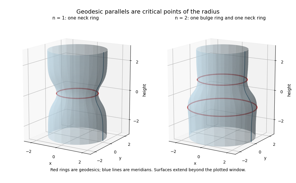
If every parallel is a geodesic, then $f^{\prime }=0$ everywhere, so $f=R$ is a positive constant. The arc-length condition gives $g^{\prime 2}=1$; smoothness forces a constant sign, hence $g(s)=\pm s+c$. The surface is a circular cylinder of radius $R$. It is a circular cylinder because the meridian is a straight line parallel to the axis.

For a variation $y+\epsilon \eta$ preserving both endpoint values and slopes, $\eta ={\eta }^{\prime }=0$ at the endpoints. The first variation isIntegrate the last term twice and the middle term once. All boundary terms vanish, givingThe fundamental lemma of the calculus of variations yields the higher-order Euler-Lagrange equationFor the present functional this becomes $1+y-y^{(4)}=0$. Its general solution is $y=-1+A\cosh x+B\sinh x+C\cos x+D\sin x$. The left endpoint gives $C=-A$ and $D=-B$. The right endpoint then givesThe coefficient determinant is $2(1+\cosh \pi )>0$, so $A=1$, $B=0$. The stationary function is $y_{\ast }(x)=-1+\cosh x-\cos x$.

For any admissible perturbation $\eta$, exact quadratic expansion, followed by the stationarity equation and integration by parts, givesApply the supplied Poincare inequality first to $\eta$, then to ${\eta }^{\prime }$, whose endpoint values also vanish:Thus $J[y_{\ast }+\eta ]\le J[y_{\ast }]$ for every admissible perturbation, proving a global maximum through the clamped second-variation inequality.

Use the Fourier transform convention $\hat{F}(k)={\int }_{\mathbb{R}}F(x)e^{-ikx}dx$, with inverse factor $1/(2\pi )$. Splitting the inverse integral at zero givesThis is the Poisson kernel for the upper half-plane at height $a$.

Take the Fourier transform in $x$ of the Laplace equation. The transformed boundary-value problem isFor $k\ne 0$ the general solution is a linear combination of $e^{|k|y}$ and $e^{-|k|y}$; the two conditions set their coefficients to zero and one respectively. At $k=0$, the solution is the constant one. Inverting therefore givesThe upper boundary holds pointwise. At the lower boundary the Dirac delta function must be interpreted distributionally: the kernel has integral one and concentrates at zero, so for every continuous compactly supported test function $h$, $\int \psi (x,y)h(x)dx\to h(0)$. This also specifies the solution in the assumed class admitting the stated Fourier transforms.

Irrotational flow permits $\mathbf{u}=\nabla \varphi$, and incompressible flow imposes $\nabla \cdot \mathbf{u}=0$, hence $\Delta \varphi =0$. In the laboratory frame, the no-penetration condition at the translating sphere is ${\partial }_r\varphi (a,\theta )=U\cos \theta$.

For separation of variables, take the angular factor $g(\theta )=\cos \theta$, which satisfies $\frac{1}{\sin \theta }(\sin \theta g^{\prime }{)}^{\prime }=-2g$. The radial equation iswith solutions $r$ and $r^{-2}$. Rest at infinity excludes the $r$ term. The normal boundary condition fixes the remaining coefficient, giving the potential flow around a translating sphereThere is no azimuthal velocity. With fluid density ${\rho }_f$, the kinetic energy isThe angular integral is $2\pi$, and the radial integral is $1/(3a^3)$, so $K_f={\rho }_f\pi a^3{U}^2/3$. Since $M=(4\pi a^3/3){\rho }_s$ and $k={\rho }_f/{\rho }_s$, $K_f=kM{U}^2/4$. Thus the added mass of a sphere is $kM/2$.

During a fall through $h$, gravity does work $Mgh$ and buoyancy does work $-kMgh$. Starting from rest, conservation of energy givesConsequently $U=\sqrt{4(1-k)gh/(2+k)}$. The mass cancels: the reduced speed comes from both buoyancy and the fluid's added mass.

A sufficient statistic is one for which the conditional distribution of the full sample, given its value, is independent of the parameter. For independent observations the likelihood is ${\prod }_{i=1}^6{p}_i^{n_i}$, depending on the data only through the counts. The factorization criterion for sufficiency therefore makes $(n_1,\dots ,n_6)$ sufficient. Directly, all ordered samples with given counts have the same probability, so their conditional distribution is uniform over the $n!/\prod n_i!$ possible arrangements, independently of the $p_i$.

The unrestricted maximum-likelihood estimator is ${\hat{p}}_i=n_i/n$. Thus the generalized likelihood-ratio test useswith zero-count terms interpreted by continuity. Reject for small $\Lambda$, equivalently large $D$.

Write $n_i=n/6+{\delta }_i$, so $\sum {\delta }_i=0$. A Taylor series expansion of $(n/6+{\delta }_i)\log (1+6{\delta }_i/n)$ gives ${\delta }_i+3{\delta }_i^2/n+O(|{\delta }_i{|}^3/n^2)$. Summing cancels the linear terms, and yieldsUnder the null hypothesis, the multinomial central limit theorem places the standardized count deviations in the five-dimensional subspace with coordinate sum zero, with identity covariance on that subspace. Their squared norm consequently tends to the chi-squared distribution with five degrees of freedom. This gives the Pearson chi-squared goodness-of-fit test.

For $T=8.12$, the asymptotic p-value is about $0.150$. The 5% critical value of ${\chi }_5^2$ is approximately $11.07$. Do not reject at the usual 5% level, or at 10%. A significance level is not specified in the paper, so an unconditional yes-or-no decision is not determined: using this approximation, rejection would require a chosen level at least about $15\%$.

Write the top row as $(u,v,5-u-v)$. The bottom row is then $(3-u,3-v,u+v-1)$, and nonnegativity becomesThe feasible set is a hexagon in this plane. Its six vertices, hence all basic feasible solutions of this transportation problem, areThere are four independent constraints; each displayed support consists of four cells forming a transportation spanning tree, so each is a nondegenerate basic solution. Conversely, a basic feasible solution is a vertex, so the hexagon enumeration is exhaustive.

For any feasible $x^{\prime }$, the proposed dual inequalities giveIf equality holds on every cell with $x_{ij}>0$, this last quantity equals $f(x)$. Hence $f(x)\le f(x^{\prime })$ for every feasible $x^{\prime }$. This is weak duality with complementary slackness.

The Northwest corner method first allocates three units to $(1,1)$, then two to $(1,2)$, one to $(2,2)$ and four to $(2,3)$:Choose ${\lambda }_1=0$, ${\lambda }_2=2$, $({\mu }_1,{\mu }_2,{\mu }_3)=(a,2,-1)$. Equality holds on its four occupied cells. The other inequalities are $-1\le 3$ and $a+2\le b$. Thus $a+2\le b$ implies that $x^{\ast }$ minimizes $f$.

The last printed clause changes from minimization to maximization. To answer that wording, use the transportation simplex algorithm for maximization, equivalently minimize the negative costs. There are only two possible entering cells at $x^{\ast }$:

Put $d=b-a$. On the feasible hexagon,If $d\le -2$, this expression is maximized by taking $u=3,v=0$, so $E$ is a global maximizer. If $d>-2$, the feasible vertex $(u,v)=(1,0)$ has objective $2(d+2)$ larger than $E$, so $E$ is not a maximizer. Nor can $C$ ever be one: comparison with $x^{\ast }$ requires $d\ge 2$, while comparison with the vertex $(0,3)$ requires $d\le -2$. Therefore one pivot to a maximizer is possible exactly when $a\ge b+2$, by entering $(1,3)$. Its reduced cost for maximization is $4>0$; the other reduced cost is $d-2\le -4$, so the improving pivot is unambiguous.