Past exam of the mathematics course of the University of Cambridge / 2020 / ib / Paper 1

Two square matrices are similar when $B=P^{-1}AP$ for some invertible matrix $P$. A Jordan normal form is a block-diagonal matrix whose blocks have one eigenvalue on the diagonal, ones on the superdiagonal, and zeros elsewhere; over an algebraically closed field every matrix is similar to such a form, unique up to reordering its Jordan blocks.

Both displayed matrices have characteristic polynomialHowever,so their eigenspace dimensions are respectively two and one. Thus $A$ has Jordan form $J_2(1)\oplus J_1(1)$, whereas $B$ has Jordan form $J_3(1)$. By uniqueness of Jordan normal form,

For an oriented smooth embedded surface, the Gauss map sends each point to its chosen unit normal. This surface is the ring torus with major radius two and minor radius one. Its outward Gauss map isOn the $y=0$ cross-section, the normal points radially away from the center of each generating circle, which gives this formula for $u=0,\pi$ and then rotational symmetry gives it for all $u$.

The upper hemisphere condition is $\sin v>0$, hence $0<v<\pi$. For this torus, the Gaussian curvature and area element areTherefore the positive outer and negative inner contributions cancel:

The boundary arcs meet at $0$ and $1$. The Möbius transformationsends these points to $0$ and infinity, sends the real boundary segment to the positive real axis, and sends the circular boundary arc to the ray of argument $-\pi /6$. Hence it maps $D\cap L$ onto the sectorThe power $\zeta =w^6$ maps this sector conformally onto the lower half-plane. Finally, the Cayley map $\zeta \mapsto (\zeta +i)/(\zeta -i)$ maps the lower half-plane onto the unit disc. Thus a requested conformal equivalence is

An operator $Q$ is Hermitian whenon its domain. Hermitian operators represent quantum observables because their expectation values and eigenvalues are real. In a normalized state,

Positivity of the norm of $(Q+i\lambda P)\psi$ for every real $\lambda$ givesThe middle expectation is real because $i[Q,P]$ is Hermitian. The discriminant of this quadratic is nonpositive, soApply this to the centered operators $Q-⟨Q{⟩}_{\psi }$ and $P-⟨P{⟩}_{\psi }$, whose commutator is still $[Q,P]$. This yields the Robertson uncertainty principleNoncommuting observables therefore cannot both have arbitrarily sharply concentrated measurement distributions in the same state.

Gaussian elimination gives the LU decompositionThe prescribed diagonal entries of $L$ are visible, and direct multiplication gives $LU=A$.

First solve $L\mathbf{y}=\mathbf{b}$ by forward substitution:Then solve $U\mathbf{x}=\mathbf{y}$ by backward substitution, obtainingDirect substitution verifies $A\mathbf{x}=\mathbf{b}$.

The likelihood contributes precision $n$ and precision-weighted mean $n\overline{X}$, while the prior contributes precision ${\tau }^2$ and precision-weighted mean ${\tau }^2\theta$. By normal-normal conjugacy with known observation variance, the posterior isThus the posterior mean isWhen $\theta =0$, its expectation under true parameter $\mu$ is $n\mu /(n+{\tau }^2)$ and its variance is $n/(n+{\tau }^2{)}^2$. Hence its frequentist mean squared error is

Write the absolute-value constraint asIntroduce slacks $s_1,s_2,s_3$. In the simplex algorithm, let $x_2$ enter and $s_2$ leave, then let $x_1$ enter and $s_3$ leave. The final dictionary isThus

For sufficiently small perturbations, the same two constraints remain active:Solving givesand therefore the perturbed optimal value is

The rank of a matrix is the dimension of its column space, equivalently the dimension of the image of a linear map represented by the matrix. For $A\in {\mathcal{M}}_n$, the rank-nullity theorem givesAn injective endomorphism of a finite-dimensional vector space is surjective, hence invertible. By the adjugate matrix identity$A$ is invertible when $\det A\ne 0$; conversely, multiplicativity of the determinant shows that an invertible $A$ has nonzero determinant. Therefore

Let $E_{ij}$ be the matrix unit with its only nonzero entry at $(i,j)$. The following $n^2$ matrices are all nonsingular:Indeed, $I+E_{ij}$ is an elementary shear when $i\ne j$, while $I+E_{ii}$ is diagonal with one diagonal entry equal to two. Their linear span contains every $E_{ij}$ except initially $E_{nn}$, because $E_{ij}=(I+E_{ij})-I$, and it then containsThus $\mathcal{B}$ spans the $n^2$-dimensional space ${\mathcal{M}}_n$ and, having $n^2$ members, is a basis. This also covers $n=1$, when $\mathcal{B}=\{I\}$.

Now let $A$ be a nonsingular zero-one matrix. If it had fewer than $n-1$ zero entries, at least two rows would contain no zero at all. Those two rows would both be the all-one row, contradicting linear independence. Hence every such matrix has at mostones. The bound is attained. Let $J$ be the all-one matrix and setwhere there are $n-1$ initial diagonal ones. If $A\mathbf{x}=0$ and $S={\sum }_j{x}_j$, the first $n-1$ row equations give $x_i=S$, while the last gives $S=0$. Hence every $x_i=0$, so $A$ is nonsingular and has exactly $n^2-n+1$ ones. Therefore

The structure theorem for finitely generated modules over a principal ideal domain applies because every Euclidean domain is a principal ideal domain. It says that a finitely generated $R$-module is isomorphic towhere the nonzero nonunits $d_i$ are unique up to multiplication by units. They are the invariant factors.

For $V_{\alpha }$, multiplication by $X$ is the linear map $\alpha$. Since $V$ is finite-dimensional over $F$, $V_{\alpha }$ is a finitely generated torsion module over the polynomial ring $F[X]$, so it has no free summand. Choosing each invariant factor $a_i$ to be monic givesThe basis $1,X,\dots ,X^{\mathrm{deg}{a}_i-1}$ of each cyclic summand makes multiplication by $X$ a companion matrix. Concatenating these bases therefore puts $\alpha$ in rational canonical form.

On $F[X]/(a_i)$, a polynomial annihilates multiplication by $X$ exactly when it is divisible by $a_i$. It follows that the minimal polynomial and characteristic polynomial areThe second identity follows blockwise from the characteristic polynomial of a companion matrix. Since every $a_i$ divides $a_k$, the product ${\chi }_{\alpha }$ annihilates every cyclic summand. Thus ${\chi }_{\alpha }(\alpha )=0$, which is the Cayley-Hamilton theorem.

For the displayed matrix, the given generators of $\ker \theta$ are the columns ofElementary row and column operations over $\mathbb{R}[X]$ give the Smith normal formConsequently the nonunit invariant factors areand, as a check,

A function $f:{\mathbb{R}}^m\to {\mathbb{R}}^r$ is differentiable at $x$ if there is a linear map $L:{\mathbb{R}}^m\to {\mathbb{R}}^r$ such thatThe map $L$, which is unique, is the derivative $f^{\prime }(x)$.

Expanding in a matrix increment $H$ givesTherefore $p$ is differentiable everywhere and

The inverse function theorem states that if $f$ is continuously differentiable near $a$ and $f^{\prime }(a)$ is invertible, then $f$ restricts to a bijection between neighbourhoods of $a$ and $f(a)$; its local inverse is continuously differentiable, with derivativeIn the normalized case $f(0)=0$ and $f^{\prime }(0)=I$, continuity of $f^{\prime }$ gives a closed ball ${\overline{B}}_r(0)$ on whichFor small $y$, define $T_y(x)=x-f(x)+y$. The mean value inequality makes $T_y$ a contraction mapping with constant $q$. If $\Vert y\Vert \le (1-q)r$, thenso $T_y$ maps the ball into itself. The contraction mapping theorem gives a unique fixed point $x_y$, and the fixed-point equation is precisely $f(x_y)=y$. Moreover,so $\Vert x_y-x_z\Vert \le \Vert y-z\Vert /(1-q)$. Thus $y\mapsto x_y$ is a continuous local inverse.

For the polynomial map in the question,The derivative is invertible, so the inverse function theorem supplies some $ϵ>0$ and a continuously differentiable $q:D_{ϵ}(I)\to {\mathcal{M}}_n$ such thatThere can be no inverse on all of ${\mathcal{M}}_n$, becauseso $p$ is not injective.

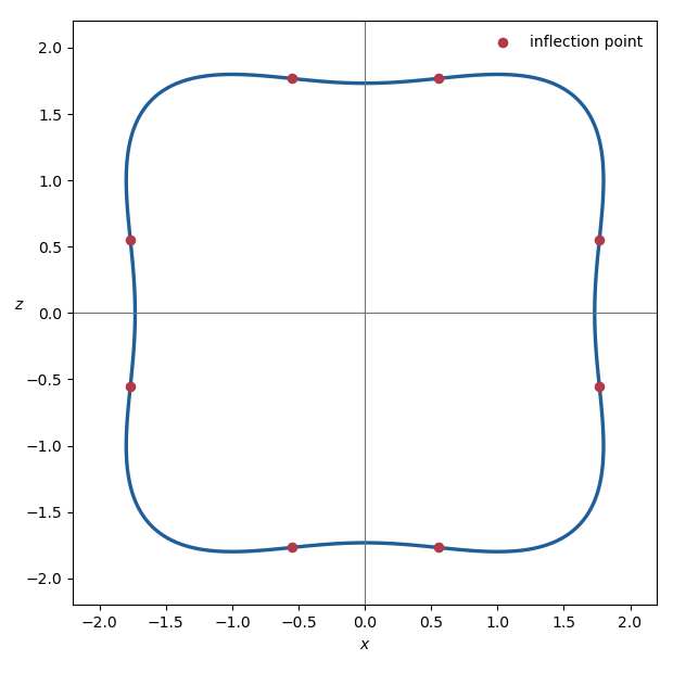
The curve is symmetric in both coordinate axes and under interchange of $x$ and $z$. Its shape, including its eight inflection points, is:

Writing $r^2=x^2+y^2$, the surface of revolution has equationLetIts gradient isIf this vanished, then $r^2\in \{0,1\}$ and $z^2\in \{0,1\}$, but at such a point $(r^2-1{)}^2+(z^2-1{)}^2\le 2$, not five. Hence zero is a regular value, and the regular level set theorem shows that $S=F^{-1}(0)$ is a smooth embedded surface.

For a surface of revolution, the two principal curvatures are the curvature of the meridian and the normal curvature of a parallel. Along $r=1$,so the normal is vertical in the meridian plane and the parallel principal curvature vanishes. Therefore the Gaussian curvature, the product of the principal curvatures, is zero there.

These are not the only zero-curvature points. The meridian itself has inflection points, at which its principal curvature vanishes. Setting $u=r^2$ and $v=z^2$, their positive squared coordinates satisfyBesides interchanging $u$ and $v$, the solution is approximatelyEach corresponding meridian inflection point sweeps out another circle on $S$, so $r=1$ does not exhaust the zero set of the Gaussian curvature.

An analytic branch of a square root determined by the branch $\ell$ isIf ${\psi }_1$ and ${\psi }_2$ are two such branches, their ratio $h={\psi }_1/{\psi }_2$ is analytic and satisfies $h^2=1$. Since a domain is connected and $h$ takes values in the discrete set $\{1,-1\}$, $h$ is constant. Thus ${\psi }_1={\psi }_2$ throughout $D$ or ${\psi }_1=-{\psi }_2$ throughout $D$.

For $z=r{e}^{i\theta }$, the principal square root isOn $D_2$, one may instead takeThe respective removed half-axes are their branch cuts.

On $\mathbb{C}\setminus [-1,1]$, defineIt is analytic there, its square is $1-z^2$, andso it is the required branch. Substitution gives, for $0<|z|<1$,The binomial series yieldshence the first three terms of the Laurent series are

Sinceits residue at zero is $-i$. Under the change of variable $z=1/\zeta$, the two orientation reversals cancel, and the residue theorem gives

In polar coordinates,With the change of radial coordinate $u=\log r$, the detection functional becomesIt is therefore $\lambda$ times ordinary path length in the $(u,\theta )$-plane. The shortest path is the line segment from $(\log A,0)$ to $(\log B,\alpha )$, soReturning to $r$ gives the logarithmic spiralIts minimum detection probability isThe functional depends only on the geometric path and not its parametrization, so tiptoeing and running give the same probability.

For the improved sensor, omit the irrelevant positive factor $\lambda$ and use the LagrangianThe coordinate $\theta$ is cyclic, so its conjugate momentum is conserved. Equivalently,is constant. Because $L$ has no explicit time dependence, the associated conservation of energy gives the constantMultiplying by $r$ and using $h=r\dot{\theta }$ gives the required equation

Expand $g$ in its Fourier sine seriesBy separation of variables, the decaying solution of Laplace equation in each half-strip has $n$th mode proportional to $e^{-k_n|x|}\sin (k_{n}y)$. Continuity at $x=0$ and integration of the equation across the Dirac delta function require the normal-derivative jumpThe jump of $C_n{e}^{-k_n|x|}$ is $-2k_n{C}_n$, so

For $g(y)=\delta (y-c)$, its Fourier coefficients areThusTranslation in $x$ gives the Dirichlet Green function for an infinite strip with source $(b,c)$:

A stationary state has the formFor a time-independent quantum observable $Q$, the global phases cancel in the expectation value:It is therefore independent of time.

For the infinite square well,The possible energy measurement results arewith respective Born rule probabilities $|c_1{|}^2$ and $|c_2{|}^2$. Normalization gives $|c_1{|}^2+|c_2{|}^2=1$.

At time $t$,The required matrix elements areConsequentlywhere the angular frequency isFinally, $2|c_1{c}_2|\le |c_1{|}^2+|c_2{|}^2=1$, so

The electric potential of a point charge $Q$ at the origin isFor the two charges forming the dipole,The first-order Taylor expansion at large $|\mathbf{x}|$ isand therefore, with the electric dipole moment $\mathbf{p}=Q\mathbf{d}$,to leading order. Taking the interaction of a second dipole with the corresponding electric field gives the stated electric dipole-dipole interaction

Let the lattice spacing be $d$ and write the central dipole asIts two horizontal neighbours have moment $p(\cos \theta ,-\sin \theta )$. For either one, the expression in parentheses, after extracting $d^{-3}$, isIts two vertical neighbours have moment $p(-\cos \theta ,\sin \theta )$, and each contributes insteadAdding all four nearest-neighbour interactions and using the Pythagorean trigonometric identity givesThe angle has cancelled, so the energy is independent of $\theta$.

For a velocity potential, $\mathbf{u}=\nabla \varphi$. The incompressible flow condition $\nabla \cdot \mathbf{u}=0$ therefore becomes Laplace equation ${\nabla }^2\varphi =0$. The Laplace equation in polar coordinates givesso positivity of $\gamma$ and $\lambda$ requiresThe velocity components areThe no-penetration boundary condition on both walls says $u_{\theta }=0$ at $\theta =0$ and $\theta =\alpha$, hence $\lambda \alpha =n\pi$. If $n\ge 2$, $\sin (n\pi \theta /\alpha )$ changes sign inside the wedge. The stated sign condition therefore selects $n=1$, and

A streamline satisfiesIntegration givesThe radius is smallest on the wedge bisector $\theta =\alpha /2$, where $\sin (\gamma \theta )=1$. Labelling that radius by $r_{\min }$ therefore givesEvery streamline arrives from infinity along one wall, reaches its closest point on the bisector, and returns to infinity along the other wall:

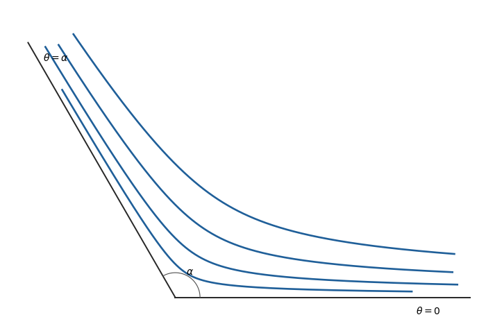
Using $\gamma =\lambda$ and the Pythagorean trigonometric identity,so the speed is independent of $\theta$. Since $\gamma =\pi /\alpha >1$,and the speed tends to zero at the vertex. The steady irrotational Bernoulli equation givesThus the fluid pressure is also independent of $\theta$, withIn particular, the pressure difference between the vertex and $r_0$ is

Define the cardinal polynomialsThey satisfy ${\ell }_k(x_i)={\delta }_{ik}$. Hence evaluating the proposed polynomial interpolation formula at $x_i$ gives $p_n(x_i)=a_i$, so the required coefficients areThe polynomial ${\sum }_k{f}_k{\ell }_k$ has degree at most $n$ and takes every prescribed value. Its uniqueness follows because the difference of two such polynomials would have $n+1$ distinct roots while having degree at most $n$.

For fixed interpolation nodes $c_0,\dots ,c_{s-1}$, interpolate any $p\in {\mathbb{P}}_{s-1}[x]$ asIntegrating shows that the unique weights making the quadrature rule exact through degree $s-1$ are

Now let the nodes be the zeros of the degree-$s$ orthogonal polynomial $q_s$. Given any $p\in {\mathbb{P}}_{2s-1}[x]$, polynomial division givesOrthogonality gives ${\int }_a^b{q}_{s}h=0$, while $q_s(c_k)=0$ makes the quadrature sum for $q_{s}h$ vanish. The rule is already exact on $r$, so it is exact on $p$. This is the defining precision property of Gaussian quadrature.