Apply the product rule in Einstein notation, using the Levi-Civita symbol to express the cross product:The third line uses a cyclic permutation of indices in the first term and an interchange of two indices in the second. Rearranging proves the divergence of a cross product identity:
Take any constant vector . Its curl is zero, so part (a) and the divergence theorem givewhere is the outward unit normal vector. The scalar triple product identity rewrites the last integrand as . Since is arbitrary, equality of these scalar products implies the vector identity
First compute the curl directly:Reflection symmetry in makes the last component integrate to zero. The middle component gives the hemisphere's volume, soFor an independent surface integral, the closed boundary consists of the curved hemisphere and its flat base. The right-hand side in part (b) is .
On the curved part use spherical coordinates with and . There,The last component has zero angular integral. The first two components giveOn the base, and the outward normal vector is . Thus . In polar coordinates its integral isThe first components cancel, and therefore both required sides equal
For the linearly damped string, substitute and divide by :Thus separation of variables givesThe fixed-end Dirichlet boundary conditions require . Nonzero solutions are , with , . Neither nor a negative spatial eigenvalue produces a nonzero function obeying both endpoint conditions.
For each sine normal mode, the temporal characteristic equation is , with roots . Since , the first modes are overdamped and all higher modes are underdamped. No integer gives critical damping.
The zero initial displacement excludes the hyperbolic cosine and cosine terms. HencewhereTo impose the initial velocity, let be its Fourier sine series coefficients. Differentiating the expansion at gives for the overdamped modes and for the underdamped modes. These determine all coefficients. Despite the hyperbolic sine, the first modes decay: , so both temporal exponential rates are negative.
Here and . LetTwo applications of integration by parts giveSolving these equations,Consequently the required amplitudes areThe stated initial velocity is nonzero at the fixed endpoints, whereas a classical solution differentiable there would require zero endpoint velocity. Thus it is understood on the open interval, or as an L2 space initial datum in the usual finite-energy solution. Its Fourier sine series takes value zero at the endpoints; this changes no initial energy or interior initial data.
For , the homogeneous solutions are . The left boundary condition selects , while boundedness at infinity selects on the right. Thus write for and for .
A unit Dirac delta distribution in the second derivative requires continuity of and a derivative jump of one:The second equation and the first give , so the Dirichlet half-line Green function for d2 minus 1 isThe second expression is also a method of images construction. Applying the Green's function to the forcing givesFor bounded forcing this is bounded, vanishes at zero and solves the equation; a bounded homogeneous solution vanishing at zero is zero, proving uniqueness. More general forcing is allowed when the integrals converge and the resulting function has the required growth. Arbitrary unbounded forcing need not admit a bounded solution; this distinction is relevant in part (b).
For , differentiation of givesThus the radial Laplacian equation reduces toBoundedness of at zero implies . Conversely, a regular reduced solution with gives finite .
There is an important qualification to the reduction in the printed question: bounded at infinity requires , not bounded . The example in part (ii) actually has , so it cannot be the bounded solution described in part (a). The differential equation and origin condition reduce as asserted, and the same Green's function can still be used with the correct growth condition. This is the radial reduction and growth at infinity distinction.
The reduced forcing is . Its exponential-weighted integrals converge, even though the resulting reduced function is not bounded. For , the Green's function formula givesFor it givesUse and to simplify this to . Dividing by yieldsThus with its continuous value at zero. At , both pieces give and , so neither a Dirac delta distribution nor its derivative is introduced at the forcing jump. The solution is bounded at both ends, with at infinity. Its reduced function confirms the growth qualification in part (i).
Using Fourier inversion with the stated convention,Hence applying the transform twice gives the duality property of the Fourier transform:The formula holds directly for rapidly decreasing smooth functions, and extends through the usual L2 space or tempered distribution formulations when absolute convergence is unavailable.
For a real nonzero , put in the Fourier transform. Reversing the integration limits when produces the absolute value:This is the scaling property of the Fourier transform. If and exists, the transformed function is constant in time; its transform is in the sense of tempered distributions, rather than an ordinary convergent Fourier integral.
The Heaviside step function restricts the integral defining the Fourier transform to , soThe convergence condition is essential. For real it means , which is the decay assumption used in the subsequent parts. At a distributional Fourier transform is needed; for negative real the defining improper integral diverges.
For , the even exponential is except for an irrelevant single value at zero. Linearity and the scaling property of the Fourier transform at giveIn particular, for positive real the transform is real and even, as expected from the symmetry of .
Set in part (d), obtaining . Apply the duality property of the Fourier transform from part (a):Therefore
For the difference of Heaviside step functions is an interval indicator, and on and zero elsewhere. Its Fourier transform isThe apparent singularity at is removable. The formula remains valid for real negative , because the original step-function difference and the oriented integral both reverse sign; for both vanish. This is the Fourier transform of an interval indicator and produces a scaled sinc function.
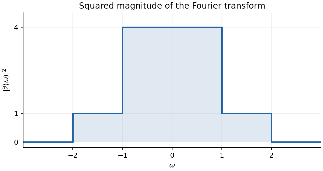
By Fourier inversion, the sinc function has Fourier transform equal to one for and zero for . Thus the two bandwidths add to giveThe requested squared-magnitude spectrum therefore has heights four and one:Values at the jump points depend on the chosen Fourier convergence convention and do not affect any integral. The graph is shown below.
Induction shows for every nonnegative integer : in a product, adjacent factors cancel. At , this is . Hence each partial sum of the matrix exponential satisfiesThe series is absolutely convergent, since a submultiplicative matrix norm bounds it by . Passing to the limit therefore proves that the matrix exponential respects similarity:No diagonalizability assumption is required.
If , then is a Hermitian matrix, because . By the finite-dimensional spectral theorem, there is a unitary matrix withThus . Since the matrix exponential respects similarity,Each diagonal entry has modulus one, so . Using ,Hence the exponential of a skew-Hermitian matrix is unitary.
The finite-dimensional spectral theorem gives a spectral decomposition of the Hermitian matrix:The matrix exponential respects similarity, soThe diagonal entries are real, so the conjugate transpose of this expression equals itself. Its eigenvalues are , provingIn particular, for any nonzero , . Thus the exponential of a Hermitian matrix is a Hermitian positive-definite matrix, even when itself has negative eigenvalues.
A square matrix is a diagonalizable matrix over a specified field if some invertible matrix makes diagonal. Equivalently, the underlying vector space has a basis of eigenvectors of .
For example,The first is already diagonal. The second has only the eigenvalue one, of algebraic multiplicity two, but its eigenspace consists of and has dimension one. It cannot supply a two-vector eigenbasis.
Every row sums to six, so is an eigenvector with eigenvalue six. Since is a real symmetric matrix, its other two eigenvalues, say , are real. The trace givesAlso, for a real symmetric matrix, is the sum of the squares of all its entries. HereThus . Together with their zero sum, this implies
By the spectral theorem for real symmetric matrices, choose an orthonormal eigenbasis corresponding to , with . Write and . This orthogonal change of coordinates givesThe plane constraint is therefore . On that plane the quadratic form vanishes exactly whenConsequently the entire set isThe two direction vectors are nonzero and not parallel, since are linearly independent. An invertible orthogonal transformation maps each full line to a full line. Thus the set consists of precisely two infinite lines through the origin.
The derivative of an analytic function must be independent of the direction of approach. Taking a real increment gives ; taking an imaginary increment givesEquality of real and imaginary parts proves the Cauchy-Riemann equations:A real harmonic function is a twice continuously differentiable function whose Laplacian vanishes. For the given logarithmic function and ,It is therefore harmonic everywhere on the punctured complex plane.
On any domain admitting a branch of the complex logarithm, chooseIts derivatives are and , as required. For example, the principal complex logarithm gives such a harmonic conjugate on the plane cut along the negative real axis.
There is no single-valued harmonic conjugate on the whole punctured plane. Indeed its putative differential would satisfywhereas a globally defined function has zero integral of its differential around a closed curve. This is the log modulus has no global harmonic conjugate on the punctured plane obstruction. Thus the conjugate requested in the question must be interpreted locally or on a cut plane.
Put . Factor out the nonzero constant in the denominator and use the geometric series:This Taylor series converges when . The simple pole at is the only finite obstruction to analyticity, whose distance from the expansion centre is five. Hence the radius of convergence is
Expand the exponential in inverse powers of :This is a Laurent series, not a Taylor series, and converges throughout . Every displayed coefficient of a negative power is nonzero, so its principal part has infinitely many terms. ThusThe residue is the coefficient of :
Divide by to put the ordinary differential equation into normalized form :The coefficients are singular at zero, butare both analytic there. This is precisely the regular singular point criterion for a second-order equation, so is a regular singular point.
Apply the Frobenius method. For , the coefficient of the lowest power comes only from ; the remaining term starts one power higher. As , this lowest coefficient gives the indicial equationTherefore the two possible characteristic exponents at a regular singular point areTheir difference is not an integer, so the two corresponding Frobenius solutions do not require a logarithmic correction.
For , the coefficient of isFactoring the bracket gives the recurrence relationFor this is . Iteration and yieldFor , the recurrence is , givingHere the double factorial products are one at , consistent with the chosen normalization. Recognizing the cosine and sine power series, for positive one may also write the two Frobenius solutions asThe constants multiplying the two independent solutions may be chosen separately.
For either exponent, the recurrence from part (c) impliesfor every finite complex . The ratio test therefore givesThe factor multiplying is an entire function in each case. For , this does not make the full Frobenius solution single-valued at zero: its square-root prefactor still requires a branch. The infinite radius refers to , not to a Taylor expansion of the branched full solution.
For fixed endpoint values and a smooth variation vanishing at the endpoints, the first variation isThe fundamental lemma of the calculus of variations gives the Euler-Lagrange equationIf is independent of , then is a cyclic coordinate, and integration givesThis is conservation of the corresponding generalized momentum.
The integrand has no explicit dependence. Thus the Euler-Lagrange equation gives the conserved transverse optical momentumAt , and the crossing slope is one, so . Solving for the positive slope gives , henceThe slopes agree at zero. The same conserved momentum holds across the interface because the refractive index is continuous and there is no point source in the variational equation.
Here a least-time ray means the minimum between the source and the receiver point selected by this ray. For those fixed endpoints, proves strict convexity in the slope, so the stationary ray is the unique minimum among graph paths. If the receiver could instead be freely placed anywhere on the line and its height were also minimized over, the horizontal ray would be faster; that different problem is incompatible with the prescribed crossing slope.
Integrate the slope in part (i), using . On the left,Its value at the interface is . On the right, integrate from the interface and enforce continuity. ThereforeBoth and are continuous at zero. The ray steepens as it approaches the interface from the left and flattens as it leaves to the right.
Retain the question's common crossing condition , and replace the slope-ratio condition of part (iii) by the specified initial slope. Then part (i) givesso . Substitution in part (ii) gives the rayIt starts at with slope , passes through with slope one, and reaches the receiver with slope . The final height isThe left-hand curvature is ; the right-hand curvature is . Thus the graph is increasing throughout, with a change from upward to downward curvature at the interface.
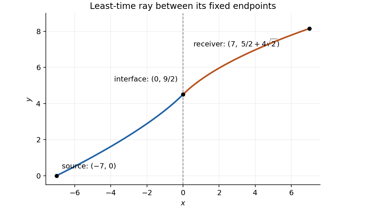


If the word “instead” were also taken to remove the common crossing condition, the initial slope alone would leave undetermined: it would give for any selected source position. The numerical answer above uses the crossing condition stated before all four subparts.
Substitute into the axisymmetric heat equation and cancel the exponential:Thus the radial ordinary differential equation and its Sturm-Liouville form areThe weight in this Sturm-Liouville problem is therefore . The outer Dirichlet boundary condition is , and the physical solution is regular at the centre. The factor in the weighted inner product is also the radial part of the polar area element.
Multiply the separated Sturm-Liouville problem by real and apply integration by parts:The outer endpoint term vanishes because . At zero, regularity gives vanishing radial flux. This can be obtained from the equation without assuming a bounded derivative: let . Since and is bounded, has a finite limit at zero. If that limit were nonzero, positive bounded thermal diffusivity would make have fixed sign and magnitude at least a constant times sufficiently near zero, contradicting bounded . Hence , and in fact . This also forces for bounded .
The boundary terms therefore vanish, provingAs usual for diffusion, is nonnegative and positive for ; the later power-law case may vanish at the centre. The argument applies in that case as well.
For a nonzero admissible radial profile define the radial diffusion Rayleigh quotientMinimizing the numerator subject to introduces a multiplier . The Euler-Lagrange equation for isThe allowed variations vanish at , and the natural condition at the centre is zero radial flux. Thus the minimum, when attained, is the smallest decay eigenvalue . Equivalently, expansion in weighted-orthogonal eigenfunctions makes a weighted average of their decay eigenvalues. The Rayleigh-Ritz variational principle therefore givesAdmissible trial functions must obey the outer boundary condition, be nonzero and have finite weighted norm and energy; they need not solve the differential equation. If the diffusion operator has no lowest eigenfunction, the same variational argument bounds the infimum of its spectrum. Existence of a fundamental diffusion mode is an additional assumption for strongly vanishing diffusivity, not a consequence of the identity alone.
For the proposed trial profile, . Its weighted energy isThe squared weighted norm isBoth are finite for and , and . Therefore the Rayleigh-Ritz variational principle givesWhen a fundamental diffusion mode exists, its decay rate is the infimum and is bounded above by this expression.
The existence qualification matters for the full range of printed in the question. For , trial functions concentrated within radius have quotient proportional to , proving the loss of a spectral gap under strongly degenerate radial diffusion. The infimum is zero and is not attained, because zero energy together with forces the zero function. Thus there is no positive lowest-mode decay rate in that case. Even at , the mode equation is : its characteristic powers are , and for every nonzero solution is unbounded at the centre. Hence the asserted bounded fundamental mode cannot be assumed for all . The trial quotient remains valid, and the next part's case has the usual fundamental mode.
For constant diffusivity, the trial Rayleigh quotient simplifies toIts derivative is , so its only positive critical point is . The second derivative is ; also the quotient diverges as or . Therefore this is the global optimum within the trial family:The two requested profiles areThe initial radial graph decreases from one at the centre to zero at the rim, has horizontal tangent at the centre, and is concave downward for . The central temperature decreases exponentially from one to zero, with initial time derivative . These are trial profiles, not exact solutions of the full heat equation. Although the radial trial function is not twice differentiable at the centre, it has finite weighted energy and belongs to the variational trial class used by the Rayleigh-Ritz variational principle.
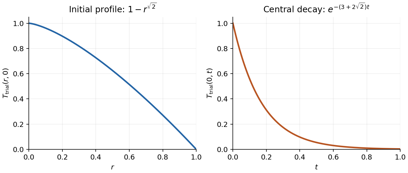
Optimal trial radial profile and its assumed exponential decay at the centre
. Details. 
Seek a positive weight such that the differential operator becomes . Matching the second derivative gives , while matching the first derivative requires . ConsequentlyChoosing the multiplicative constant to be one givesThis is Sturm-Liouville form with zero potential term. Multiply the equations for by , subtract, and integrate. The Lagrange identity for a Sturm-Liouville operator givesThe boundary expression vanishes because and the functions and their derivatives are finite. Since are distinct, their eigenvalues are distinct, provingThe endpoint singularities of the weight are integrable, so these weighted inner products exist.
For , a constant solution and its normalization give . For , substitute : the equation gives , and the normalization gives . For , put . Comparing coefficients gives and ; then fixes . ThusThese are the first three Chebyshev polynomials. For their squared weighted norms, use , which converts into :More generally, makes their orthogonality the usual cosine orthogonality.
Articles were limited to the first 100 out of 183 total.
Articles by others on the same topic
There are currently no matching articles.