Past exam of the options I course of the University of Oxford / 2009 (XMAT 4303, AO1)

Options I, Honour School of Mathematics Part A, Trinity Term; Wednesday 24 June 2009, 9.30am–12.30pm. The nine-page source is preserved in a private editable transcription, including its intact cover and all nineteen questions. It was supplied through the past-papers disclosure, at original Part A bundle pages 132–140. No exact worked-answer advertisement was found in the bounded availability check.

The splitting field is the smallest subfield of $\mathbb{C}$ containing $\mathbb{Q}$ and all the roots of a polynomial under consideration. Equivalently it is generated over $\mathbb{Q}$ by those roots, and the polynomial splits there into linear factors.

Put ${\zeta }_6=e^{\pi i/3}$. All sixth roots of unity are powers of ${\zeta }_6$, so the required splitting field isIndeed ${\zeta }_6=(1+\sqrt{-3})/2$, and conversely $\sqrt{-3}=2{\zeta }_6-1$. Its field extension degree is two.

The polynomial identityshows that the roots are the ninth roots of unity which are not third roots. These are precisely the primitive ninth roots of unity, all powers of ${\zeta }_9=e^{2\pi i/9}$. Thus the splitting field is $\mathbb{Q}({\zeta }_9)$. The supplied irreducibility statement makes the displayed degree-six polynomial the minimal polynomial of ${\zeta }_9$, giving

Write $g(x)=x^6+x^3+1$. The second polynomial is $g(-x)$. Negating the roots of a polynomial does not change the field generated by them: each original root is minus a new root, and conversely. Hence this splitting field is again $\mathbb{Q}({\zeta }_9)$ and its field extension degree is six. Equivalently, it is the cyclotomic field $\mathbb{Q}({\zeta }_{18})=\mathbb{Q}({\zeta }_9)$, since ${\zeta }_{18}=-{\zeta }_9^5$.

A solvable group has a finite subnormal series from the identity to the group with abelian group factors. An equivalent definition uses the derived series: set $G^{(0)}=G$ and $G^{(j+1)}=[G^{(j)},G^{(j)}]$; the series must reach the identity. For completeness, an abelian-factor series forces successive derived subgroups into its successive terms, while a terminating derived series itself supplies such a series.

If $H\le G$, induction gives $H^{(j)}\le G^{(j)}$: every commutator of elements of $H^{(j)}$ is also a commutator in $G^{(j)}$. Thus termination for $G$ implies termination for $H$, proving that every subgroup of a solvable group is solvable.

In $S_4$, useThe Klein four-group is invariant under conjugation in $S_4$; the other normality assertions follow from the alternating group being the kernel of the sign map. The quotient group factors are $V_4,C_3,C_2$, all abelian. Hence $S_4$ is solvable.

For the last example take $A_5\times C_2$. Its subgroup $\{1\}\times C_2$ is nontrivial, proper and normal, so the product is not a simple group. Projection onto $A_5$ is surjective, and every quotient of a solvable group is solvable, because a homomorphism carries each derived subgroup onto the derived subgroup of its image. But the nonabelian simple group $A_5$ has $A_5^{\prime }=A_5$: its derived subgroup is nontrivial and normal. Thus the product is not solvable either. One standard justification of the simplicity used here is that the nonidentity conjugacy class sizes of $A_5$ are $15,20,12,12$; no proper nontrivial union with the identity has size dividing $60$, as a normal subgroup would require by Lagrange's theorem for finite groups.

Fermat's little theorem says that for a prime number $p$ and any integer $a$,If $p\nmid a$, cancellation gives the equivalent statement $a^{p-1}\equiv 1(\mathrm{mod}p)$.

Wilson's theorem states that an integer $p>1$ is a prime number if and only ifIn particular this holds for every prime, including $p=2$.

Apply Fermat's little theorem and Wilson's theorem in the ring of integers modulo n with modulus $p$. They giveA vanishing modular congruence modulo $p$ is precisely divisibility by $p$, so both divisibilities hold, without requiring $p\nmid a$.

Because the primes are distinct, Fermat's little theorem gives $q^{p-1}\equiv 1(\mathrm{mod}p)$ and $p^{q-1}\equiv 1(\mathrm{mod}q)$. The other term in each modulus vanishes. ThereforeThe distinct primes are coprime, so their product divides this integer. Hence

The Lebesgue outer measure can be defined byA null set has $m^{\ast }(E)=0$, equivalently it admits such a cover of total length below every positive $\epsilon$.

The usual Cantor set is the intersection of the sets obtained from $[0,1]$ by repeatedly removing every open middle third. At stage $n$ there are $2^n$ closed intervals of length $3^{-n}$. Enlarge them slightly to open intervals whose total added length is below $\epsilon$. Thus $m^{\ast }(C)\le (2/3{)}^n+\epsilon$ for every $n$ and $\epsilon >0$, proving $m^{\ast }(C)=0$.

For the different deletion rule in this problem, let $L_n$ be the total length of the stage-$n$ intervals. Removing the stated fraction from each component givesFor $n\ge 1$ the telescoping product simplifies toBecause $K\subseteq K_n$, the same finite interval-enlargement argument gives $m^{\ast }(K)\le L_n$. Taking the limit provesOnly interval covers and their lengths were used; no continuity theorem for integrals is needed.

One version of dominated differentiation under the integral sign is the following. Let the parameter range be open. Suppose $f(\cdot ,y)$ is integrable, ${\partial }_{y}f(x,y)$ exists for almost every $x$, and near each parameter value its absolute value is bounded by an integrable function of $x$ independent of $y$. ThenThis follows by applying the dominated convergence theorem to difference quotients, bounded by that same integrable function through the mean value theorem.

On any compact parameter interval $0<y\le B$, the original integrand is bounded by $B/(1+x^4)$, using $|\sin (x^{2}y)|\le B{x}^2$. Its first and second parameter derivatives areTheir absolute values are bounded respectively by $(1+x^4{)}^{-1}$ and $x^2/(1+x^4)$, both integrable on $(0,\infty )$. Applying the theorem twice proves that $F$ is twice differentiable and givesThis last integral is absolutely convergent: its integrand is bounded near zero and bounded by $x^{-2}$ at infinity. Substituting $t=x\sqrt{y}$ yieldsThe expression for $c$ is finite and independent of $y$, which is all that is required.

The family $\mathcal{F}$ of closed sets contains $\varnothing$ and $X$, is closed under arbitrary intersection, and is closed under finite union. Conversely these axioms define a topology by declaring the complements of the members of $\mathcal{F}$ to be the open sets.

The map is continuous when the preimage $f^{-1}(U)$ is open in $X$ for every open set $U$ in $Y$. Equivalently the preimage of every closed set in $Y$ is closed in $X$, since preimages commute with complementation.

Convergence of a sequence to $\ell$ means that every open neighbourhood $U$ of $\ell$ contains all sufficiently late terms: there is $N$ such that $x_n\in U$ for all $n\ge N$. The threshold may depend on $U$.

Both $\varnothing$ and $X$ satisfy the condition. For an arbitrary intersection of members, either every member contains $a$, in which case the intersection contains $a$, or one does not, in which case that member is countable and so is the intersection. The empty intersection is $X$.

For a finite union, either a member contains $a$, so the union does too, or all members omit $a$ and are countable, so their finite union is countable. Thus the closed set axioms hold and define a topology. This is a Fortissimo space: every point other than $a$ is isolated, while the open neighbourhoods of $a$ have countable complement.

Let $S=\{x:f(x)\ne f(a)\}$, which is countable. For any closed set $C\subseteq \mathbb{R}$, consider its preimage. If $f(a)\in C$, then $a\in f^{-1}(C)$ and that preimage is closed by definition. If $f(a)\notin C$, then $f^{-1}(C)\subseteq S$, so it is countable and again closed. Therefore every closed set has a closed preimage, proving continuity.

Set $S=\{x_n:n\in \mathbb{N},x_n\ne \ell \}$. This is a countable set, hence a closed set in the stated topology, and $\ell \notin S$. Consequently $X\setminus S$ is an open neighbourhood of $\ell$. By convergence of a sequence, all sufficiently late terms lie outside $S$. A sequence term outside $S$ must equal $\ell$. Thus the sequence is eventually constant, and only finitely many indices have $x_n\ne \ell$.

A subset $A$ is compact when every open cover of $A$ has a finite subcover. This may be stated using sets open in the ambient space or using the subspace topology on $A$; the definitions agree because every subspace-open set is the intersection of $A$ with an ambient-open set.

Let $(U_i{)}_{i\in I}$ be an open cover of $f(X)$, with the sets open in $Y$. The preimages $f^{-1}(U_i)$ form an open cover of $X$, because $f$ is continuous. By compactness, finitely many of these preimages cover $X$. Their corresponding sets $U_i$ cover $f(X)$, providing a finite subcover. Hence the continuous image is compact.

The family contains the empty set and the entire real line. The intersection of two proper nonempty members isso it is closed under finite intersection. For an arbitrary nonempty family of proper rays, put $c={\inf }_i{a}_i$. If the thresholds are unbounded below, the union is $\mathbb{R}$; otherwise the union is $(c,\infty )$. In the latter case $c$ itself is in no ray, and every point greater than $c$ lies above some threshold, proving the equality. Empty unions and unions involving $\mathbb{R}$ cause no difficulty. Thus arbitrary unions also belong to the family, establishing the topology axioms.

If $m=\min A$, any open cover contains a member containing $m$. Such a member is either $\mathbb{R}$ or a ray $(a,\infty )$ with $a<m$. It therefore contains every element of $A$, so that single member is already a subcover.

Conversely suppose $A$ is nonempty and has no smallest element. Thenis an open cover of $A$: for any $x\in A$, the lack of a minimum gives an $a\in A$ below $x$. A nonempty finite subcollection has union $(a_0,\infty )$, where $a_0$ is the smallest of its thresholds. It misses $a_0\in A$. The empty subcollection cannot cover nonempty $A$ either. Hence there is no finite subcover, and $A$ is not compact. Thus compactness is equivalent to having a smallest element.

There are real Lagrange multipliers ${\lambda }_1,{\lambda }_2$ such thatEquivalently $Dg(x_0)={\lambda }^{T}Df(x_0)$. The rank assumption says the two constraint gradients are linearly independent; it rules out an abnormal constraint point.

Use constraints $h_1=x^2/4+y^2+z^2-1$ and $h_2=x+y-z$. Both constraints and the objective are continuously differentiable. The feasible set is a nonempty closed subset of a bounded ellipsoid, hence compact, so the extreme value theorem guarantees both extrema.

The gradients $(x/2,2y,2z)$ and $(1,1,-1)$ are independent everywhere feasible. If the first were $t$ times the second, then $x=2t$, $y=t/2$, $z=-t/2$. The plane constraint would give $3t=0$, forcing the origin, which is not on the ellipsoid. Thus the Lagrange multiplier theorem applies at every feasible point.

Its equations areHere $\lambda \ne 0$, since otherwise the first two equations require $\mu =1=2$. Subtract twice the first equation from the second, and use $\mu =2\lambda z$ and $z=x+y$; the result is $0=-3\lambda x$, so $x=0$. Then $z=y$ and the ellipsoid gives $y=\pm 1/\sqrt{2}$. The only candidates are therefore $(0,\pm 1/\sqrt{2},\pm 1/\sqrt{2})$, with matching signs. Consequently

Take a smooth variation $u+\epsilon \eta$ with $\eta$ vanishing on the boundary; compactly supported test functions suffice for the interior equation. At an extremum, the first variation is zero:Integration by parts removes the derivatives from $\eta$. The boundary terms vanish, givingThe fundamental lemma of the calculus of variations gives the Euler-Lagrange equationThis is the classical equation for sufficiently smooth admissible extrema; for weaker regularity the first-variation identity supplies its weak form.

For the squared-gradient integrand, the equation is $2(u_{xx}+u_{yy}+u_{zz})=0$, namely the Laplace equation. Put $u_0=ax+by+cz$ and write any admissible function as $u=u_0+v$, with $v=0$ on the boundary. The energy identity isBy the divergence theorem, the middle integral is ${\int }_{\partial V}v(a,b,c)\cdot ndS=0$; equivalently it vanishes by weak integration by parts for zero-trace functions. The final term is nonnegative and vanishes at $v=0$. Thus this is a global minimum, not merely a stationary value:

With $\mathbf{d}={\mathbf{q}}_1-{\mathbf{q}}_2$ and $r=|\mathbf{d}|$, the Lagrangian isAt configurations with $r>0$, the Euler-Lagrange equations giveThese formulas apply on the differentiable part of the potential; collision configurations require any additional smooth extension of $f(|\mathbf{d}|)$ to be specified. Summing the equations givesso the total linear momentum is conserved. The total energy isDifferentiating, the two interacting forces do work $-f^{\prime }(r)\dot{r}$, while the potential derivative is $f^{\prime }(r)\dot{r}$ and particle three contributes no force term. Hence $\dot{E}=0$. Both total momentum and total energy are conserved.

For the first particle, the derivative of its angular momentum about the origin is its torque:This need not vanish. For example take $f(r)=r^2/2$ and instantaneous positions ${\mathbf{q}}_1=(1,0,0)$, ${\mathbf{q}}_2=(0,1,0)$; the torque is $(0,0,1)$. Therefore it is not conserved in general, although it is in special configurations or for a constant potential.

The third particle is force-free, so its torque about the origin vanishes:Thus this angular momentum is conserved.

Let $\mathbf{F}$ be the force on particle one, so the force on particle two is $-\mathbf{F}$, with $\mathbf{F}$ parallel to ${\mathbf{q}}_1-{\mathbf{q}}_2$. The combined torque isHence the combined angular momentum of particles one and two is conserved. Centrality of their interaction, in addition to equal and opposite forces, is what makes this torque sum zero.

For a field point in the plane of the loop, both the directed line element $d\mathbf{s}$ and the displacement $\mathbf{r}-\mathbf{s}$ lie in that plane. Their cross product is normal to it, so every term of the Biot-Savart law is normal, and their integral is normal as well. This argument also allows the field to vanish at particular points.

Choose the loop in the $xy$-plane with centre at the origin and let positive current be counterclockwise as seen from $+z$. On its lower side, write $\mathbf{s}=(t,-a,0)$, $-a\le t\le a$, soThat side contributesAll four contributions have the same direction and size by rotation. Thuswhere $\mathbf{n}$ follows the right-hand rule for the current.

For a planar incompressible flow, a stream function satisfies $u={\psi }_y$, $v=-{\psi }_x$. A velocity potential satisfies $u={\varphi }_x$, $v={\varphi }_y$ where the flow is irrotational; such a potential exists locally, and globally on a simply connected nonsingular region. The irrotational flow condition is $v_x-u_y=0$. Where both exist, the Cauchy-Riemann equations make the complex potential $w=\varphi +i\psi$ analytic with $w^{\prime }=u-iv$.

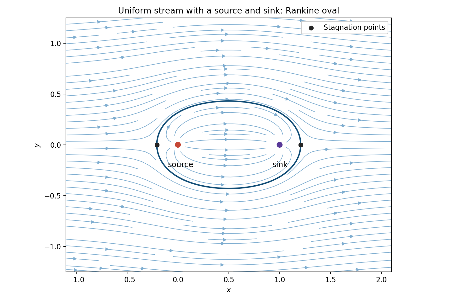
For the logarithmic potential, write $z-z_0=r{e}^{i\theta }$. ThenThe outward volume flux per unit span across a circle is $2\pi r{u}_r=m$. Hence it is a line source of strength $m$. The potential may use local logarithm branches; its velocity is single-valued away from the source.

By superposition, the full flow hasFor positive $m$ and $U$, the stagnation points areThey are real, one upstream of the source and one downstream of the sink. Away from the singularities, streamlines are level curves ofThe zero level through the two stagnation points contains an upper and a lower separating curve, symmetric about the real axis and about $x=1/2$. Together they bound a Rankine oval. Flow inside goes from source to sink; the external stream divides around this oval and tends to horizontal flow far away. This also specifies the sketch for every positive parameter ratio; the figure illustrates one ratio.

For the isolated line vortex, use polar coordinates $z=r{e}^{i\theta }$ to obtainThus for nonzero $\Gamma$ the streamlines are circles and their counterclockwise circulation is $2\pi r{u}_{\theta }=\Gamma$. If $\Gamma =0$ the fluid is stationary and the streamline description degenerates.

Place an opposite image vortex at $z=-1$. The method of images givesOn $z=iy$, the distances to the two vortex positions agree, so $\psi =-(\Gamma /2\pi )\log (|z-1|/|z+1|)=0$. Hence the wall is a streamline. Directly the wall velocity has $u=0$ andFor the stipulated steady flow, Bernoulli's equation in the irrotational fluid outside the vortex core givesThe force exerted by the fluid on this wall points in the $-x$ direction for positive pressure. Relative to uniform pressure $p_{\infty }$, however, its change is in the $+x$ direction. Using the supplied integral, the force change per unit span isThus the wall is attracted towards the vortex, with this magnitude if the other side remains at $p_{\infty }$. Subtracting the uniform pressure is essential for an infinite wall. A freely moving vortex would translate parallel to the wall under its image-induced velocity; the calculation here is for the stated steady vortex configuration, with its position held fixed.

Pointwise,Taking expectations and dividing by $a^2>0$ gives the second-moment form of Markov's inequality:

The inverse transformation is $x=uv$, $y=u(1-v)$, with support $u>0$, $0<v<1$. Its absolute Jacobian determinant isThe original joint probability density function, by independence, is ${\lambda }^2{e}^{-\lambda (x+y)}$ on the positive quadrant. The change of variables formula therefore givesIntegrating over $v$ givesthe gamma distribution of shape two and rate $\lambda$. Integrating over $u$ gives $f_V(v)=1$ on $(0,1)$. The factorization also shows that $U$ and $V$ are independent.

The preceding marginal calculation makes each $V_i$ uniformly distributed on $(0,1)$, with expectation $1/2$ and variance $1/12$. By independence,Apply part (a) to the centred random variable $Z=S_n/n-1/2$ to obtainThis is Chebyshev's inequality in this setting.

For $n=0$, the conditional transition probabilities are ${\delta }_{ij}$, the entries of $P^0=I$; for $n=1$ the assertion is the definition of $P$. For the induction step, condition on the state at time $n$ and use the Markov property and time-homogeneity:The countable sum is justified by the law of total probability; all terms are nonnegative. Thus the formula follows for every $n$ by induction. It is the Chapman-Kolmogorov equation for repeated one-step transitions.

Let $u_n=\mathbb{P}(X_n=1\mid X_0=1)$. Conditioning on $X_n$ givesThe fixed value is $b/(a+b)$. Subtracting it and iterating the scalar recurrence yieldsThe formula includes $n=0$. If $a+b=1$, its value at $n=0$ is interpreted directly as $u_0=1$, while $u_n=b$ for all $n\ge 1$. Since $|1-a-b|<1$, the limiting probability is $b/(a+b)$.

At the first step, the chain enters state two with probability $p$ and state four with probability $1-p$. The classes $\{2,3\}$ and $\{4,5\}$ are closed and disjoint, so only the first branch can reach state three. On $\{2,3\}$ the transition matrix is exactly the two-state matrix from part (b). Thus after the remaining $n-1$ steps, the probability of the second state in that class isFor $n=1$ it is zero, as the original matrix requires; this statement covers the zero-base exponent case without ambiguity.

State one is left after one step and never revisited. The eventual probability mass in the closed class $\{4,5\}$ isWithin this class the stationary distribution is $(b/(a+b),a/(a+b))$, because the balance equation is $a{\pi }_4=b{\pi }_5$. The two-state recurrence shows convergence from either starting state, since $|1-a-b|<1$. The other closed class never reaches state five. Therefore

By continuity of the cumulative distribution function and nonnegativity, $F(0)=0$; strict increase and $F(x)\to 1$ allow inversion for every $0<t<1$. The probability integral transform follows fromThus $F(X)$ is uniformly distributed on $(0,1)$.

The order statistics arrange the sample increasingly: $X_{(1)}\le \cdots \le X_{(n)}$. Strict monotonicity means $F(X_{(i)})$ is the $i$th order statistic of $n$ independent uniform variables. Its density isobtained by choosing the $i-1$ observations below $t$ and the $n-i$ above it. This is the beta distribution with parameters $i,n+1-i$, soFor the given log-logistic distribution, rearrangement givesConsequently plot $y_i=\log (i/(n+1-i))$ vertically against $x_i^{\ast }=\log X_{(i)}$ horizontally. Under a good fit, replacing $F(X_{(i)})$ by its plotting position $i/(n+1)$ gives an approximate straight line withThis is a diagnostic probability plot, rather than an assertion that the expectation of the nonlinear transformed order statistic equals that transformed plotting position. Positive observations occur almost surely under the model.