Source paper: Oxford public source archive, member 2017/A10288W1_CP2_Sept_2017.pdf. The cover dates this resit to 5 September 2017. Lettered scopes below distinguish separately marked paragraphs where the source supplies no letters. All four Section B options are covered.
In a source-free vacuum, the Maxwell equations in SI arewhere and are the vacuum permittivity and vacuum permeability. Take the curl of the last equation, substitute Faraday's law of induction, and use the curl of the curl identity:The zero divergence therefore gives the wave equationFor a propagating plane wave, write . The wave equation gives , and Gauss's law for magnetism gives . Thus the oscillating magnetic field is a transverse wave: it is perpendicular to the propagation wavevector. A static background magnetic field, if present, is separate from this propagating component.
The central point charge and spherical boundaries give a spherically symmetric charge distribution. A conductor in electrostatic equilibrium has zero electric field within its material. Consequently a spherical Gaussian surface inside the metal encloses zero net electric charge, so the inner surface carries . The shell's prescribed total electric charge then leaves on its outer surface. Gauss's law givesThe electric field is singular at the ideal central point charge. At each charged surface the normal component has distinct one-sided limits, as required by the electrostatic boundary conditions at a conductor. Spherical symmetry makes the outer surface charge density uniform:
For the uniform space charge in a grounded spherical cavity, grounding sets the metal's electric potential to zero. With no external sources and zero electric potential at infinity, the exterior electric potential is also zero by the uniqueness theorem for the electrostatic potential. The original shell electric charge is no longer fixed: electric charge can flow to or from earth.
Inside the cavity, Gauss's law gives . Integrating the electric field inward from the zero boundary electric potential givesThe inner surface carries , where , and the outer surface carries zero net electric charge. Only the cavity contributes to the final electrostatic energy:The same result follows from ; the conductor's surface charge contributes zero because its electric potential is zero. This is the final stored electrostatic energy, not the change from the earlier central-charge configuration, whose ideal point charge has divergent self-energy.
Use the parallel-plate capacitor approximation, neglecting the fringing field of a capacitor. With plate area , the initial capacitance and opposite plate electric charges areAfter the electric battery is disconnected, the isolated plate electric charges stay fixed. Doubling the separation halves the capacitance. The quasistatic pulling work is the increase of electrostatic energy:The final electric potential difference is thereforeAn electron released at rest gains kinetic energy , where is the positive elementary charge. Neglecting radiation and the negligible perturbation caused by this one electron, conservation of energy givesThis is , so the nonrelativistic kinetic energy is adequate. The circular plates have finite radii; the numerical results are leading parallel-plate capacitor values rather than exact finite-plate capacitances.
The current density is the moving charge density times its velocity:For a cylindrical Gaussian surface of radius and length , cylindrical symmetry makes the electric field radial. Gauss's law gives . A circular Ampère's circuital law contour encloses electric current , giving . HenceThe right-hand rule fixes the positive azimuthal direction of the magnetic field for positive electric charge moving along . Both the electric field and the magnetic field vanish on the axis. These are the steady long-cylinder electric field and magnetic field; end effects and changes of the prescribed beam distribution are excluded.
For normal incidence on a diffraction grating, adjacent grooves contribute a path difference . Constructive interference occurs when the grating equation holds. Thus the groove spacing isAn allowed propagating diffraction order must have . ThereforeThe fifth diffraction order is the highest geometrically permitted order for this wavelength. Its actual brightness depends on groove shape and the single-slit diffraction envelope, which the source does not specify; geometric permission alone does not guarantee a bright observable maximum.
The original diagram has an ideal electric battery feeding series resistors of above the tapping point and below it. The long battery bar is positive, so terminal is above terminal in electric potential. With an open circuit at the output, the internal electric current is . The voltage divider therefore givesFor the Thévenin resistance, suppress the ideal voltage source by replacing it with a short circuit. The two resistors are then in parallel as seen from :By Thévenin's theorem, the terminal voltage under an outward load electric current is . Consequentlyflowing through an external short circuit from to . Directly shorting the original terminals bypasses the resistor and leaves across , independently confirming the result.
The integral and differential forms of Gauss's law in electrostatics areHere is a closed surface bounding a volume , is its outward area vector, is the electric field, is total volume charge density, and is enclosed electric charge. The divergence theorem converts one form to the other. For ideal sheets or point charges, interpret the differential equation with their distributional charge densities.
Write the uniform surface charge density on the annulus as , and let be signed distance along its axis. A ring of radius and width contains electric charge . Its transverse electric field components cancel in pairs, and its electric potential is . Setting and integrating gives the axial field of a uniformly charged annulus:At , each element's electric field cancels that of the diametrically opposite element, so . There is no surface charge at the centre because ; the axis electric field is continuous there.
For positive and , differentiate the signed axial electric field:Its stationary condition is . Factoring with and givesThe derivative starts positive, has exactly one positive zero and is negative at large , so this is the positive-side maximum. For either sign of , the electric field magnitude has equal maxima at . As , the thin-ring limit is .
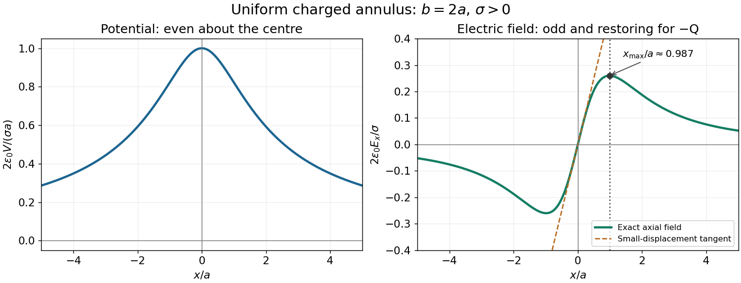
Axial potential and electric field of a uniformly charged annulus
. Original dimensionless curves for and positive surface charge density. The dotted line marks the calculated positive-side maximum of the electric field; the dashed tangent shows its linear behaviour near the centre. Details.Let be the sliding point charge's mass. Expanding the axial field of a uniformly charged annulus for givesIts electric charge is , so its electric force points toward the centre. Newton's second law becomesTo leading order this is simple harmonic motion, withThe mass is an additional parameter, since the source supplies no numerical value. The constraint is essential: stability along the axis does not imply unconstrained three-dimensional trapping by a static electric field.
For a steady filamentary electric current , the Biot-Savart law isHere is the observation position, the source position, points in the direction of positive electric current, and is the vacuum permeability. A circular loop has centre magnetic field : the cross product has magnitude and a constant axial direction, and .
Introduce the constant signed angular velocity about the positive axis. A ring's electric charge crosses any radial cut once per rotation, so its electric current is . Adding loop contributions yields the magnetic field of a rotating charged annulus:The direction follows the right-hand rule for positive electric charge; reversing either or reverses the magnetic field. The source supplies no rotation rate, so the answer necessarily retains .
Take from the negative to the positive point charge. Their electric dipole moment is . Place them at and use the superposition principle for the electric potential:For , the first-order Taylor expansion of the reciprocal distances givesto leading electric dipole order. In spherical coordinates aligned with , the gradient gives , and . ThusEquivalently, the electric dipole field is . The omitted terms vanish relative to these leading expressions as .
The method of images replaces a conductor's induced surface charge by suitable fictitious image charges located outside the physical region in which the electric field is sought. Choose them so that the combined electric potential satisfies the specified conductor boundary values, has the required behaviour at infinity, and has the correct physical sources. The uniqueness theorem for the electrostatic potential then identifies this constructed electric potential with the physical solution in that region.
For an infinite grounded conducting plane at , a point charge at with has an image charge at . Distances to the pair are equal on the plane, so their electric potentials cancel there. This construction determines the electric field above the plane; below it the actual conductor has constant electric potential and zero electric field, rather than the fictitious image's continuation.
Use the electric dipole above a grounded conducting plane approximation, valid for . Let point upward, and choose . Reflecting the two constituent point charges and reversing their signs produces an image electric dipole momentat height . Thus the parallel electric dipole moment reverses and the normal one is unchanged. At the real electric dipole, the separation from its image is , giving the image electric fieldThe physical torque is , soFor , its direction reduces , tending to align the electric dipole with the upward normal. In general it favours either normal orientation; a perfectly parallel orientation has zero torque but is unstable to tilting.
The conductor-response potential energy includes one half of the real-image interaction:This factor accounts for the induced surface charge changing as the physical source is assembled. Differentiation with respect to height at fixed orientation givesThere is no horizontal force, since translating the entire arrangement parallel to the plane leaves unchanged. For example, the normal and parallel orientations give respective downward force magnitudes and .
A single physical point charge induces total plane electric charge . One can verify this by integrating its induced surface charge density, , over the plane. The two physical electric charges therefore induce opposite totals, givingThe local surface charge density is generally nonzero. The zero total holds for the finite neutral pair as well as its ideal electric dipole limit.
Fermat's principle states that the travel time, or equivalently the optical path length in a stationary medium, is stationary under small variations of the path with endpoints held fixed. It need not be a global minimum.
Let a light ray join a point at height above a plane interface to a point at depth below it, with horizontal separation . If the crossing point is horizontally from the first endpoint, its optical path length isSetting its derivative to zero givesThe two geometric ratios are the sines of the incident and refracted angles, measured from the interface normal vector. Hence Snell's law is
The paraxial approximation restricts light rays to small slopes relative to the optical axis, so and geometric lengths can be expanded to second order in height. Treat the source's optical lens as a thin lens located at , with and small surface slopes.
For positive real conjugate distances , the collapsed-plane geometric path has lengthTo thin-element accuracy, a segment of this path lies inside the optical lens, replacing the same length of air. The geometric air path is , the material path is , and the optical path length and travel time are thereforeThis distinguishes geometric length from optical path length; adding to without subtracting the replaced air would count that segment twice.
For a nonaxial light ray, Fermat's principle gives and henceThe focal length is obtained with the incident object at infinity:The constant thickness supplies a common delay but does not change the leading focal length. Since has units of inverse length, this formula has the correct dimensions. These are thin lens results; paraxial approximation alone does not remove finite-thickness corrections in a general thick lens.
Substituting the stated refractive index and thickness coefficient, , givesThe thin lens equation then givesThe positive image distance places a real image on the outgoing side of the optical lens, at . The object is beyond the focal point, so outgoing light rays actually converge there rather than only their backward extensions meeting.
Use phasors with time dependence . The electrical impedance is the complex number relating the sinusoidal voltage and electric current: is their amplitude ratio and is the voltage phase relative to the electric current. The component laws giveThus the resistor has zero relative phase, the capacitor voltage lags its electric current by , and the inductor voltage leads its electric current by . The ideal capacitor and inductor store and return energy; the real electrical impedance of the resistor describes dissipation.
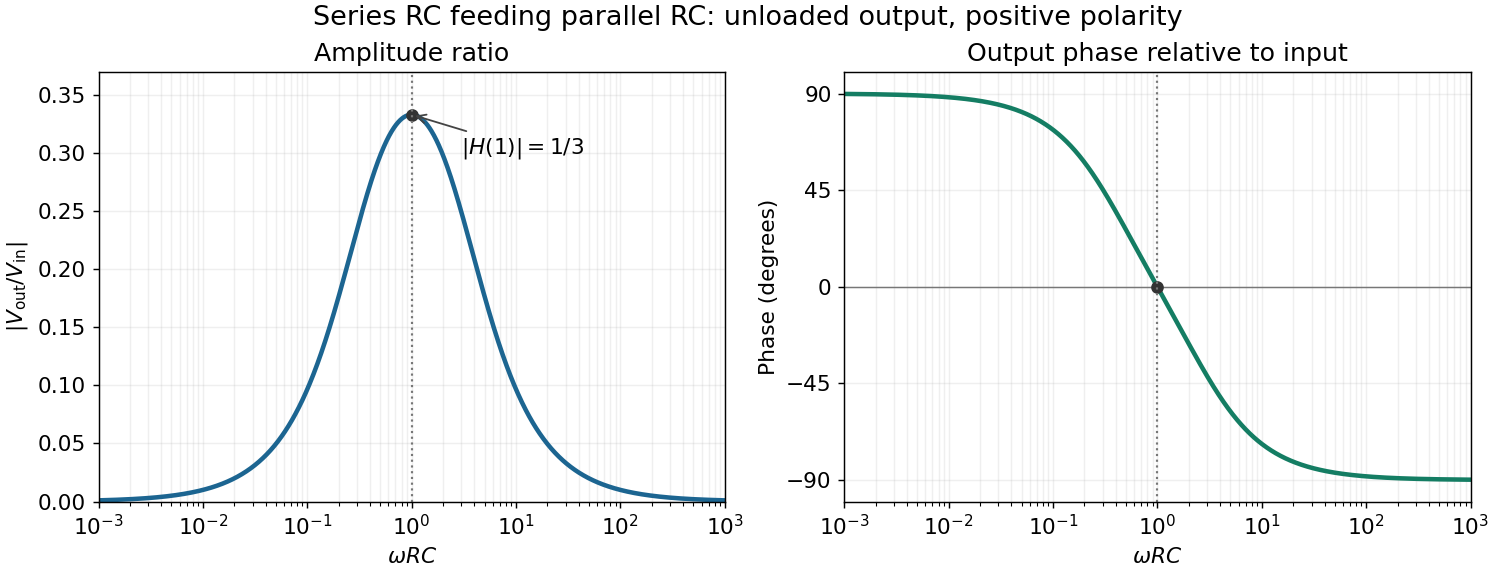
The original diagram's upper arm is a series resistor and capacitor; its lower arm is a parallel resistor and capacitor. The output is the upper-minus-lower voltage across that parallel arm. Assume an ideal input voltage source and an unloaded output. Their electrical impedances areFor this series-parallel RC band-pass filter, the voltage divider gives, with ,Taking the real part of yields the steady outputInitial charging contributes decaying transients if the source is switched on at a finite time; the displayed expression is the sinusoidal steady state. The output polarity matters: reversing the indicated output voltage would multiply by .
For positive angular frequency, the squared amplitude response of the series-parallel RC band-pass filter isIts denominator is minimized exactly when , soThis is a band-pass filter maximum produced entirely by the two RC arms; the drawn electrical circuit contains no inductor. The low- and high-frequency limits areThus the output amplitude tends to zero linearly with at low frequency and as at high frequency. In real time,The upper series capacitor suppresses low frequencies, while the lower shunt capacitor suppresses high frequencies.
In the chosen phasor convention, output phase minus input phase isThe real part of the denominator is positive, so this principal arctangent is continuous throughout the positive-frequency range. Below , the output leads the input, approaching at low frequency. Above , it lags, approaching at high frequency. At the maximum,The input and output are in phase there, with the positive one-third voltage ratio found above.


Articles by others on the same topic
There are currently no matching articles.