For the intended ideal Venturi effect, take steady flow, incompressible flow, negligible viscous losses, and the same height at the two stations shown. The Bernoulli equation along a streamline givesUsing water mass density ,Thus the outlet pressure is lower by . The increased kinetic energy per unit volume comes from the drop in pressure.
The source's assumption of laminar flow alone does not imply negligible viscosity or losses. The numerical result uses the usual lossless Bernoulli equation approximation, with the quoted speeds interpreted as representative streamline speeds. A real tube with significant viscous losses requires additional data; in a uniform-velocity energy balance its pressure drop would include an extra positive loss term.
The principal moments of inertia are the eigenvalues of the symmetric inertia tensor. In units of , its characteristic determinant isTherefore the requested algebraic answer isAn orthonormal basis of principal axes is , , and ; the last two span the degenerate eigenspace and may be replaced by any orthonormal basis of it.
There is a physical inconsistency in calling the supplied matrix a rigid body's inertia tensor. The moment-of-inertia triangle inequalities require each principal moment to be no greater than the sum of the other two. Here . In principal coordinates, cannot be negative for a nonnegative mass distribution. Thus the eigenvalue calculation is well defined, but no ordinary rigid mass distribution realizes this tensor. The positive second-moment matrix test for an inertia tensor makes the same obstruction explicit.
Use local east, north and upward unit vectors at the equator, with Earth's rotation . The parcel starts at rest relative to the ground. To first order in , its unperturbed vertical velocity is and its fall time from height isThe Coriolis acceleration is . Since north crossed with downward points west, its negative points east:Integrating with gives the equatorial Coriolis deflection in free fall,For , and , andThis neglects air resistance, variation of over the fall, and terms of order . The measured local already includes the background centrifugal correction. “Stationary” is interpreted as hovering above a fixed ground location, not being stationary in an inertial frame.
Under a uniform compressive pressure , each normal stress is . The isotropic Hooke's law gives each longitudinal strain asThus . By the definition of bulk modulus, , so the isotropic elastic modulus relation isPositive finite Young's modulus and bulk modulus requireThe incompressible limit is with at finite . If positivity of the shear modulus is also imposed, the full stable isotropic range is . Negative Poisson's ratio is not ruled out; the displayed bulk-modulus relation alone supplies the upper bound.
For the intended reversible adiabatic process, an ideal gas obeys . A monatomic gas has heat capacity ratio , soThe required extra assumption is that “adiabatic” denotes the usual quasistatic isentropic process. Absence of heat transfer alone would not fix the final temperature: an ideal gas undergoing free expansion into vacuum is also adiabatic but leaves its temperature unchanged.
- Kepler's first law: a bound planetary orbit is an ellipse with the central attracting body at one focus.
- Kepler's second law: the line from that focus to the planet sweeps equal areas in equal times, equivalent to constant areal velocity.
- Kepler's third law: the squared orbital period is proportional to the cube of the semi-major axis, when the orbiting mass is negligible.
The first law includes a circular Kepler orbit as a special case. The third-law constant is the same for bodies orbiting the same dominant mass.
Choose zero gravitational potential energy at infinite separation. The spacecraft's conserved total orbital energy isAt periapsis and apoapsis, the radial velocity vanishes, so the velocity is perpendicular to the radius. The conserved angular momentum magnitude is thereforeThe angular momentum vector is normal to the fixed orbital plane. The respective units are joules and . These expressions use Newtonian gravity and the approximation .
Eliminate using the angular momentum expressions from part (b):HenceFor distinct turning radii, factor the difference of squares and cancel the common factor to obtainThe circular Kepler orbit case is recovered continuously by setting , giving . Combining this with the energy expression also gives for the transfer ellipse.
Use a Hohmann transfer orbit. At the initial radius , make a short prograde burn parallel to the existing velocity. The increased speed changes the circular Kepler orbit into an elliptic orbit whose periapsis is the burn point and whose apoapsis lies on the desired larger circle. Coast for half the transfer orbital period to apoapsis.
At that point the transfer velocity is again tangent to the target circle, but its magnitude is smaller than the circular speed there. A second short prograde burn raises it to the required circular speed. Thus both burns increase the instantaneous speed and preserve its direction at the burn, even though the final circular speed is lower than the original one. During the coast the spacecraft loses kinetic energy while gaining gravitational potential energy.
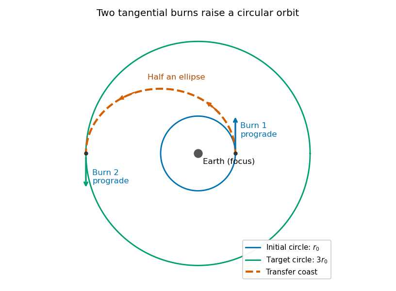
Original transfer-orbit construction for the later example with outer radius three times the inner radius; arrows show the two prograde burns
. Details. 
The figure illustrates for the subsequent parts, but the same construction works for any larger target radius. The impulsive approximation neglects the distance travelled during each burn and keeps both circles and the transfer ellipse coplanar.
The original circular Kepler orbit has . For the transfer ellipse, set , in part (c):The first required speed increase is . Under the question's negligible-mass-change fuel model, fuel use is proportional to the magnitude of the impulse. Since the full fuel supply corresponds to ,This is the stated “about a quarter” of the original fuel supply. It is an instance of the Hohmann transfer impulse fractions; no variable-mass rocket model is required under the stipulated assumptions.
At transfer apoapsis, angular momentum conservation givesThe desired circular Kepler orbit has speed . Thusof the original fuel supply is used in the second burn. This is about of the fuel remaining after the first burn. The total transfer consumes of the original supply, leaving about . The two positive impulse magnitudes are added for the fuel budget, even though their directions at opposite ends of the orbit differ.
A normal mode of a linearized mechanical system is a motion in which every generalized displacement oscillates at a single common angular frequency, with fixed relative amplitudes and phases. In coordinates , an undamped oscillatory mode may be writtenwhere the amplitude vector is fixed; negative components describe relative phase . An arbitrary small motion is a linear combination of the normal modes when the mode vectors form a complete basis.
Let be each sphere's moment of inertia about the fibre, and let be the common fibre filament torsional stiffness, so a length exerts restoring torque . The single-sphere torsion pendulum obeysFor the two coupled torsional pendulums, the upper fibre has twist and the joining fibre has relative twist . The joining fibre exerts equal and opposite torques on the two spheres:Using the measured givesThe fibre's own rotational inertia and damping are neglected, so its twists supply elastic torques without additional dynamic coordinates.
Set and use normal mode amplitudes , with real physical displacements obtained at the end. In units of , the stiffness matrix isWriting , the eigenvalue condition isThereforeFor finite positive fibre lengths both eigenvalues are positive. The corresponding amplitude ratio isThe lower normal mode has the spheres twisting in the same sense, and the higher one has opposite signs of angular displacement.
In terms of ,Both curves decrease monotonically: with , , while . The limits, including their leading approach, areThus the limiting squared angular frequencies are and infinity for short joining fibre, and zero and for very long joining fibre. For orientation, at the values are . The high-frequency curve stays above and the low-frequency curve below .
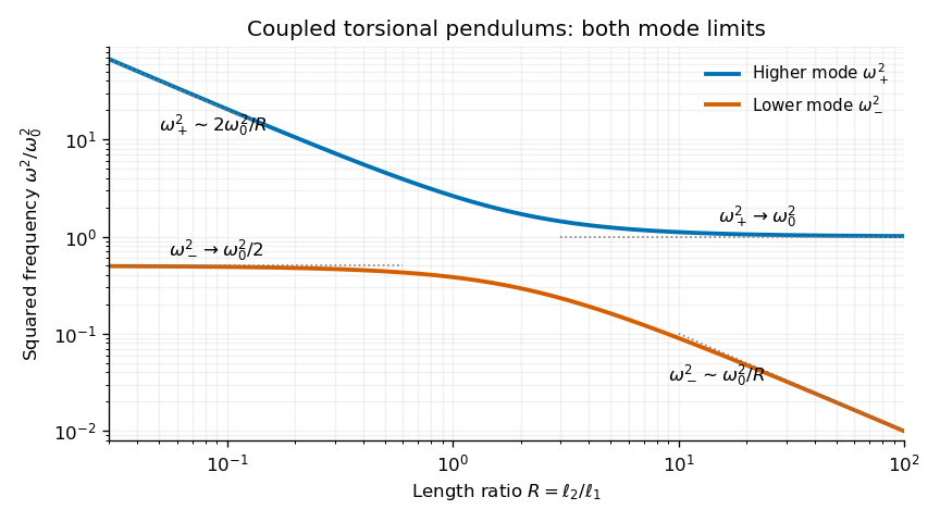
Calculated squared normal-mode frequencies versus fibre-length ratio; both axes are logarithmic to show all four asymptotic limits
. Details. 
As , the short joining fibre is very stiff and the lower normal mode has . The spheres therefore behave as one torsional load with combined moment of inertia , suspended by the upper fibre of torsion constant . Its angular frequency satisfiesThe high-frequency opposite-twist mode costs increasingly large elastic energy and moves to arbitrarily high frequency in the massless-fibre model.
As , the joining fibre is very compliant. In the higher normal mode the lower sphere scarcely moves: the amplitude ratio tends to . The upper sphere approaches the original single torsion pendulum, givingThe other mode is then a slow twist of the almost freely suspended lower sphere. These interpretations assume the formal limits do not invalidate the thin massless-fibre approximation.
In a linear isotropic dielectric of relative permittivity , the electric displacement field and electric field satisfyHere denotes the free charge density called in the question. For spatially constant , these also give . Equivalently, and . The electric displacement field has units and the electric field has units .
The local equations determine the fields once their geometry and boundary conditions are specified; a density value alone does not determine a unique vector field without that information.
Let point from medium 1 to medium 2. Integrate over a thin Gaussian pillbox crossing the interface. As its thickness tends to zero, the side contribution vanishes and any free surface charge density givesApply to a thin rectangular loop spanning the same interface. Its short sides vanish in the limit, so the tangential electric field is continuous:For a clean dielectric interface with no free surface charge density, these electrostatic interface boundary conditions reduce to and . In particular ; the normal electric field itself need not be continuous. Bound polarization charge is already incorporated into .
Consider a long uniform length of a coaxial cylindrical capacitor, with permittivity and inner-cylinder charge per unit length . A cylindrical Gaussian surface givesThe electric potential difference isThus its capacitance per unit length is .
In the partially filled coaxial capacitor, the vacuum section of length and the dielectric section of length share the same two conductors and hence the same electric potential difference. They are electrically in parallel, not in series. The radial electric field is tangent to the axial dielectric interface, consistent with the boundary condition in part (b). Adding their charges givesThis is the leading long-capacitor expression, neglecting end and interface-fringing corrections. The stated supports a long filled section; treating the other section as uniform also requires it to be well away from the end regions when those corrections matter.
Let increasing overlap mean that the dielectric moves farther into the capacitor. Its capacitance derivative isAt fixed electric potential difference , the capacitor energy rises by , but the voltage source supplies electrical work . The difference is available as mechanical work :The dielectric insertion force at fixed voltage is thereforeFor the usual , it pulls the dielectric inward, increasing ; its magnitude is constant within the long-overlap approximation. In the original longitudinal diagram this is to the left. The units are newtons, since is energy per length. Differentiating the field energy alone with a minus sign at fixed would miss the source contribution; the correct fixed-voltage capacitor energy balance is essential.
Use for the magnitude of charge on either plate. The fully filled capacitance is , while the initial value is given in part (c). At the same fixed electric potential difference,For and positive , this is an increase in the positive plate's electric charge magnitude, supplied by the voltage source; the negative plate acquires an equal opposite change. The net free charge of the two-plate capacitor remains zero. Thus “charge on the capacitor” has its usual circuit meaning, not the algebraic sum over both plates.
The electric field is approximately radial in the long interior, but near an electrode end its lines spread into a fringing field of a capacitor. The electric field magnitude falls on moving outward through that end region. The dielectric's induced electric dipoles experience a net force toward the stronger field, pulling the material into the capacitor. For a weakly perturbing polarizable element this is expressed by , with positive electric polarizability .
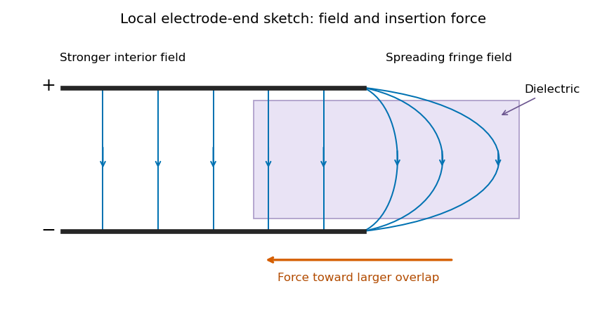
Local schematic of field lines at an electrode end and dielectric insertion; this illustrates the fringe rather than the full coaxial geometry
. Details. 
In the sketch the field lines run from the positive electrode to the negative one, curving outward near their ends. The material is attracted toward the interior where the field is stronger. A perfectly uniform interior field by itself would not give a longitudinal dipole-gradient force; the end region is essential to the local explanation. Neglecting its small contribution to the total capacitance does not justify omitting the finite insertion force that it transmits. The energy argument of part (d) gives that force without needing the detailed fringe solution.
For a steady filamentary electric current in vacuum, the Biot-Savart law isThe line element points with conventional electric current, and the cross product fixes the magnetic flux density direction by the right-hand rule.
As an application, an infinitely long straight wire has circular symmetry about its axis. At perpendicular distance ,Its direction follows the right-hand rule. The following part applies the same law to a circular current loop.
Parameterize the loop by and choose positive electric current counterclockwise as seen from . At the observation point ,The numerator of the Biot-Savart law isThe distance is constant round the loop. The transverse terms integrate to zero, while the axial term integrates to . HenceFor use below, define the undisturbed magnetic field intensity . This distinguishes the applied field from the internal field after adding the magnetic sample.
The printed formula has a physical problem for the specified geometry. Let be the linear magnetic susceptibility, where is the source's relative magnetic permeability. The constitutive equation is , not in general .
For a small uniformly magnetized ellipsoid with its principal axis along the applied field, include its demagnetizing field through the SI demagnetizing factor :Solving givesA slender rod aligned along the field has as its aspect ratio grows. Its ideal slender-rod limit at fixed is thereforeprovided . A finite cylinder generally has nonuniform magnetization, so an ellipsoidal shape factor is an approximation, and its aspect ratio is needed for a more precise correction. Small sample length compared with the field-variation scale makes approximately uniform across it; that condition does not set the demagnetizing factor to one.
The source's displayed instead follows from , the thin-plate limit with field normal to the plate. It can also be obtained by imposing , but that identification is not justified for a thin rod parallel to the field. Consequently the requested extra cannot honestly be derived from the stated rod geometry. The next part gives both the shape-consistent result and the force conditional on using the printed magnetisation.
In the small-body approximation, write , with . The induced magnetic dipole moment is . Its effective interaction potential energy at fixed source current isThe factor accounts for inducing the moment: differentiating as if the moment were permanent would double the force. Equivalently, the instantaneous dipole force is . Thus the force on a small linearly magnetizable body isFrom part (b), . HenceFor the ideal slender rod, . If the source's printed magnetisation is imposed instead, its corresponding conditional answer isFor and , both expressions point toward the loop, where the applied magnetic field is stronger; for the direction reverses toward the loop plane. A material with diamagnetism, , reverses this attraction. The force is in newtons, since a magnetic dipole moment times a field gradient has units . Both formulas assume linear response, negligible saturation and approximately uniform applied field across the sample.
For a linear induced response, reversing reverses and the sample magnetization, while also reversing the field gradient. Their product in therefore keeps the same sign and magnitude:This is also explicit in the dependence in part (d), for both the shape-consistent and printed alternatives. The conclusion assumes no independent permanent moment, remanence or hysteresis; those would require a different response model.
Changing shape changes the demagnetizing field, and hence the magnetization induced by the same applied magnetic field intensity. For a small linear sample in the ellipsoid approximation, the force magnitude scales withFor , a more elongated body aligned with the field has smaller and a stronger response. A sphere has , giving ; a very thin plate with field normal to it has , giving . Thus an axially slender rod generally experiences a stronger attraction than a sphere or a transverse thin plate of the same material and volume, within the linear uniform-applied-field approximation.
The shape response is precisely why the factor in part (c) cannot apply universally to every small magnetic body. Orientation also matters through the appropriate principal demagnetizing factor; for general nonellipsoidal bodies the internal field is not uniform and a single scalar correction need not be exact.
Articles by others on the same topic
There are currently no matching articles.