All optional physics questions are covered. The protein application in 1(c) and the bacterial application in 2(a) are TODO: user-deferred biology; the ordinary physics portions are retained.
Use the amphiphile packing parameter , where is tail volume, the effective head-group area and the maximum tail extension. The conventional cylindrical-micelle window is . Its upper limit follows directly from cylindrical micelle geometry: a long core of radius has volume-to-area ratio , so . The spherical packing limit is ; above it a filled spherical core cannot accommodate the assumed head-group area and chain length.
Inverting both positive inequalities givesThus the useful estimate is a head-group area of approximately –. If phase-boundary configurations are excluded, use strict inequalities. These endpoints are geometric morphology crossovers, rather than exact thermodynamic phase boundaries: chain conformations and head-group interactions also affect which micelle minimizes the free energy. The supplied molecular volume is interpreted as the tail-core volume required by this packing model.[ref]
Theory of self-assembly of hydrocarbon amphiphiles by Jacob N. Israelachvili and others. 1976, aggregate packing theory; cylindrical and spherical core constraints
For an equilibrium contact angle measured through the liquid, Young's equation balances the tangential interfacial forces:The pure-ethanol measurement therefore fixes the solid–vapour surface energy asThe inferred surface energy is , equivalently . The equality of these units follows because creating interfacial area costs energy.
For the equal-fraction mixture, the stated linear relations give and . Holding the solid–vapour surface energy fixed,The small decrease in increases the numerator of Young's equation, but the increase in has the larger relative effect and reduces . Consequently the contact angle increases and the mixture wets the surface less well. This inference uses equilibrium wetting on an unchanged smooth solid; a changing surface composition or contact-angle hysteresis would require additional measurements.
TODO: user-deferred biology. The protein-specific haemoglobin displacement requested here is deferred; no species-specific numerical answer has been calculated.
The ordinary physics is Stokes settling velocity. For a generic isolated rigid sphere of radius , particle mass density and surrounding-fluid mass density , balance the buoyancy-corrected body force against Stokes law:Here is the dynamic viscosity. If the effective acceleration is approximately constant over the displacement and the terminal regime has been reached, . In an actual centrifuge , so a sufficiently large radial change requires integrating instead of assuming constant . This generic relation does not resolve the deferred biological application.
TODO: user-deferred biology. The bacterial-motion application is deferred. The following covers the Reynolds number and its general fluid-mechanical implications.
The Reynolds numbercompares advective inertia with viscous force on a specified length scale and velocity scale . Here is fluid mass density, is dynamic viscosity and is kinematic viscosity. In the Navier-Stokes equation, advective acceleration scales as , while the viscous term per unit mass scales as ; their ratio is Reynolds number.
When and unsteady fluid inertia is also negligible, the incompressible flow equations reduce to Stokes flow:Thus pressure, applied body forces and viscous stresses balance at each instant. For a translating rigid sphere, drag is proportional to velocity, , rather than the inertial scale . Given the same instantaneous geometry, reversing the imposed boundary velocities reverses the Stokes flow; there is no fluid-inertial coasting in this approximation. This statement concerns the fluid limit and does not discard a separately significant particle inertia.
A low steady Reynolds number alone does not justify dropping rapid unsteady acceleration. For forcing frequency , the additional dimensionless ratio is . No organism-specific sizes, velocities or propulsion mechanism are assumed here.
The Flory interaction parameter measures the excess cost of unlike segment contacts. In a simple lattice with coordination number , contact energies and temperature ,A positive Flory interaction parameter penalizes unlike contacts; a negative value favors them. Mixing still depends on the balance with entropy of mixing, rather than the sign of alone.
For two polymers of degrees of polymerization , let be the volume fraction of species . The binary Flory-Huggins polymer blend has mixing free energy per lattice siteThe logarithmic terms favor mixing. Their factors and arise because an entire chain translates as one object; connecting many segments greatly reduces the mixing entropy per segment. Hence long polymers can demix for a much smaller positive Flory interaction parameter than small molecules.
For composition-independent , the local stability criterion isPositive curvature means stability to small composition fluctuations, zero curvature locates the spinodal, and negative curvature means spontaneous growth of fluctuations. Actual two-phase coexistence is determined by the common-tangent construction, or equality of both species' chemical potentials; its boundary is the binodal. A locally stable but globally unfavourable homogeneous mixture can lie between the binodal and spinodal.
Setting the second and third derivatives of to zero givesFor the symmetric Flory-Huggins polymer blend, and . For a polymer solution with and long chains of species , , consistent with the theta solvent limit. An effective Flory interaction parameter can depend on temperature and composition; in the simple energetic case , heating encourages mixing, but that temperature trend is not universal.
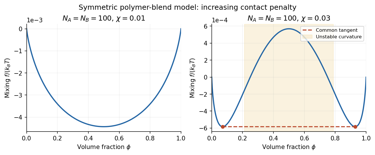
The original illustration uses stipulated . At the mixing free energy is convex, whereas at a central unstable region appears. The horizontal common-tangent construction in the latter case joins the symmetric coexisting compositions; its contacts differ from the spinodal boundaries. These are model curves, not supplied experimental data.
The critical micelle concentration is the approximate surfactant concentration above which added amphiphile predominantly joins micelles. Isolated amphiphiles expose their tails to the surrounding solvent; aggregation can reduce the unfavorable exposure, while losing translational entropy and incurring head-group and chain-packing costs. The favored aggregate minimizes the total free energy.
A mass-action model of micellization makes the concentration dependence explicit. For aggregation of monomers into one micelle, equilibrium requiresThe dimensionless thermodynamic activities therefore obeyFor a large aggregation number , a modest increase in monomer activity produces a steep increase in micelle abundance. In an ideal dilute approximation with the same reference concentration for both species, the amphiphile balance isWell below the crossover almost every amphiphile is isolated. Above it, most additional amphiphile enters micelles, so the free-monomer concentration rises only slowly. It is not exactly constant for a finite , and a small aggregate population can exist below the nominal critical micelle concentration. The experimentally sharp change is an association crossover, not an assertion that aggregation is absolutely absent below one concentration.
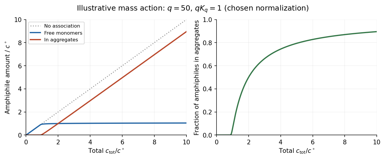
In the original illustrative model, and after choosing the arbitrary reference concentration. The normalization is a teaching choice, not a measured critical micelle concentration. The monomer curve flattens relative to total concentration, while the aggregated fraction rises rapidly.
An experimental critical micelle concentration can be estimated from a change of slope in surface tension against the logarithm of total surfactant concentration, as interfacial coverage approaches saturation and bulk aggregation becomes important. Changes in electrical conductivity for ionic surfactants, or in light scattering, supply other probes. Different observables can give slightly different operational values because the crossover has finite width. Molecular structure, temperature and ionic conditions affect the balance of chemical potentials; screening charged head groups can reduce repulsion and favor aggregation, but no universal sign of the temperature dependence should be assumed.
A colloid has dispersed constituents whose relevant dimensions are mesoscopic: roughly to in at least one direction. Interfaces and Brownian motion are consequently important. The size range is a useful convention, not a sharp boundary separating all physical behaviour. A sol of fine silicon dioxide particles in water illustrates solid in liquid; an oil-in-water emulsion illustrates liquid in another immiscible liquid; and a foam illustrates gas dispersed in a liquid, with thin intervening films supplying the small structural dimension. A colloid need not be a thermodynamic equilibrium state.[ref]
Definition and classification of colloids by International Union of Pure and Applied Chemistry. Definition and classification of colloids: approximate size range, colloidal dispersions, sols, emulsions and foams
Unprotected particles attract through Van der Waals forces. For two equal spheres of radius with a small surface gap , the near-contact van der Waals attraction of spheres iswhere the Hamaker constant is positive for the attractive case. The large number of interacting constituent molecules can give a well much deeper than , even though individual molecular attractions are weak. Brownian motion brings particles together, and a sufficiently deep attractive well makes separation unlikely. This gives particle aggregation; solid particles can remain distinct within a cluster rather than merging into one continuous solid. Emulsion droplets can additionally coalesce if the separating film ruptures.
Charge stabilization of colloids supplies a repulsive barrier. Like-charged surfaces carry compensating counterions and electric double layers; bringing the layers together costs free energy. DLVO theory combines this repulsion with Van der Waals forces. A barrier large compared with can make aggregation slow, even when sticking would lower the final free energy. Adding salt generally shortens the Debye–Hückel screening length and can lower the barrier; surface charge regulation and specific ion interactions also matter. A negatively charged particle and a positively charged particle need not repel.
Steric stabilization instead coats each particle with adsorbed or grafted polymer chains. In a good solvent, overlap and compression of these layers raise the osmotic pressure and reduce chain entropy, opposing close contact. Electrosteric stabilization combines the two mechanisms. Dense, securely bound layers matter: incomplete adsorption can allow polymer bridging, while nonadsorbing dissolved polymers can create an attractive depletion force. Poor solvent quality can collapse a protective layer. Reducing the density mismatch slows sedimentation but does not remove the interparticle attraction, so uniform suspension and resistance to aggregation are different requirements.
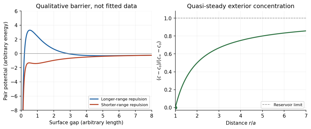


The left panel is an original qualitative potential with arbitrary coefficients: it illustrates a barrier and its reduction by shorter-ranged repulsion, without fitting an experimental DLVO theory curve or extrapolating the continuum attraction to molecular contact. The right panel plots the derived quasi-steady concentration profile in dimensionless variables.
In diffusion-controlled growth, attachment is rapid and delivery through the surrounding medium is the bottleneck. The growing surface depletes the neighboring solute, so a substantial concentration gradient develops. In reaction-controlled growth, arrival is fast compared with incorporation; many arrivals fail to attach, and the surface concentration stays near the reservoir value. The analogous distinction for particle aggregation is between near-unit sticking probability in diffusion-limited cluster aggregation and barrier-suppressed sticking in reaction-limited cluster aggregation. Here the subsequent calculation concerns accretion onto one growing particle, rather than a collision kernel for two mobile clusters.
The printed time-dependent equation is the diffusion equation, not the usual Poisson equation. For constant diffusion coefficient , no bulk sources and negligible advection, Fick's laws give the number flux . Local conservation of mass, expressed here as conservation of the accreting constituent, then givesAn arbitrary time-independent exterior profile does not solve the full moving-boundary problem exactly. The required elementary result uses a quasi-steady approximation: diffusion establishes the exterior profile much faster than the particle radius changes. At each instantaneous radius , set . Thus the exterior field solves the homogeneous Laplace equation,Two integrations give . The two boundary conditions fixFor growth, , so the profile increases outwards. Its radial flux is negative, and the positive inward arrival rate isA material density is needed to turn an arrival rate into a radial velocity. Introduce the constant constituent number density inside the particle, using the same units as . The sharp-interface balance, neglecting exterior advection, isThe difference accounts for material already present in the volume swept by the growing interface. In the usual dilute-feed approximation , it can be replaced by . With constant reservoir and surface concentrations, integration from radius gives the constant-reservoir diffusion-controlled particle growth lawConsequently when the growth contribution dominates . For a finite seed at the literal limit , the increment is instead initially proportional to . Here “early time” means before appreciable reservoir depletion or interactions with other particles, while already beyond the rapid initial establishment of the diffusion field. Indeed, the ratio of diffusion-adjustment time to radial-growth time is ; small supersaturation relative to the particle density makes the quasi-steady approximation self-consistent. No initial concentration field was specified, so an exact transient solution is not uniquely determined.
For comparison, let a finite surface-attachment coefficient be and the equilibrium surface concentration be . In the dilute-feed approximation, the Robin boundary condition givesFor this recovers transport control; for , the surface-reaction-controlled particle growth has approximately constant . Thus reaction control gives , in contrast to the diffusion-controlled square-radius law. No numerical or is supplied or needed for these scaling results.
Polydispersity means that a sample contains chains of different molar masses or lengths. Let count chains with molar mass . The number-average molar mass gives every chain equal weight, while the weight-average molar mass weights a chain population by its contribution to total mass:Writing makes the latter interpretation explicit: . Large chains therefore influence more strongly. If brackets denote an average over chain number,The ratio is molar-mass dispersity, conventionally written Đ. It equals one only when every chain has the same molar mass. Different distributions can share the same ratio, so it does not specify the full distribution.
For a freely jointed chain, write the end-to-end vector as the sum of independently oriented steps , each of fixed length . Isotropy gives , and independence gives for . HenceThe root-mean-square end-to-end distance of a polymer chain is , although the mean vector is zero. Its polymer contour length is , an upper bound on extension; it is not the typical unforced end-to-end length.
Stiffness correlates neighboring bond directions, so the discarded cross terms need not vanish. A freely rotating chain fixes the angle between successive forward bond vectors but leaves torsion uniformly distributed. Set , so . ThenFor a chain long compared with its orientational correlation range, the characteristic ratio of a freely rotating chain approaches . Positive forward persistence increases the mean-square size and gives the Kuhn length of a freely rotating chain . A chemical internal bond angle is supplementary to the forward-vector angle used here, so substituting that internal angle requires . For at fixed , the finite sum tends to , the rigid-rod result; taking the long-chain limit first would incorrectly predict an unbounded size. Real torsional energy preferences can be represented by a rotational isomeric state model, with weighted torsional states and correlations beyond independent free rotations.
A worm-like chain describes continuously varying local orientation. For unit tangent and bending stiffness , its elastic energy is . In three spatial dimensions the persistence length is andSince , integrating the tangent correlation gives the end-to-end distance of a worm-like chain:For , expansion gives , approaching a straight rod. For , it gives , the long-chain ideal chain result with Kuhn length . These models isolate stiffness; long-range excluded volume can additionally swell an isolated chain in a good solvent. When coarse-graining, a chemical repeat count and a count of independent statistical steps must not be silently interchanged.
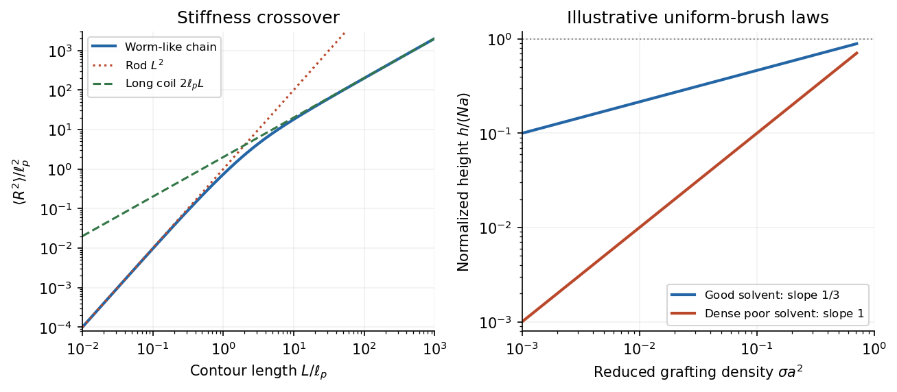
Stiff-chain crossover and distinct polymer brush density scalings
. Details. 
The first panel shows the exact worm-like chain crossover between a rod and a long flexible coil. The second compares original normalized scaling curves for a uniform polymer brush; their prefactors have been chosen for illustration and do not fit the exam's experimental points.
For a good solvent, consider long flexible grafted polymer chains with grafting density and lateral spacing . At high coverage, is smaller than the isolated coil size, and adjacent chains cannot retain their unperturbed conformations. A scaling model divides each chain into concentration blobs of diameter . Inside one blob the chain retains good-solvent statistics,using the Flory approximation exponent . The blobs per chain form a stretched sequence approximately normal to the surface. The good-solvent brush height therefore obeysHere and refer to consistently chosen effective segments, whose microscopic properties are held fixed as chain length changes. The result is a scaling law with an undetermined order-one prefactor, not a fully specified height in nanometres.
A complementary free-energy balance per chain iswhere is effective segment excluded volume. The first term is the chain entropy cost of stretching and the second is the cost of crowding segments into a layer of volume per chain. Minimization gives ; with it recovers the same height. The blob argument incorporates good-solvent correlations more directly. Both descriptions require overlapping chains, many segments per chain, and heights below the polymer contour length; the power law cannot be extrapolated to infinite grafting density.
In the printed experimental graph, the vertical axis is and the horizontal axis is . The approximately straight trend through the origin therefore means . Since and is proportional to chain length for a fixed repeat chemistry,The dashed guide rises by roughly – vertical units over six horizontal units, corresponding to of order per unit of the plotted . This is an approximate graphical slope, not a fitted material constant; the graph does not specify a numerical monomer count or a repeat-unit volume from which an absolute brush height could independently be calculated.
The poor-solvent brush height has a simple volume argument. Let be the volume per repeat and the roughly fixed polymer volume fraction within a dense uniform layer. There are repeats per substrate area, soFor fixed poor-solvent conditions, is approximately independent of and , giving the observed linear grafting-density dependence. Polymer–polymer contacts are favored and the layer becomes relatively compact; in a good solvent, favorable solvent contact and segment repulsion instead produce a swollen layer whose stretching and osmotic costs balance at the weaker dependence. Sparse isolated polymer globules or lateral segregation fall outside the uniform-brush model.
The cited experimental paper's abstract independently reports these two scaling laws, but identifies polydimethylsiloxane chains on porous silicon dioxide, rather than the polystyrene system named in the exam. The solution uses the printed axes to infer the exponents and does not treat that material identification as verified experimental provenance.[ref]
Characterization of the brush regime for grafted polymer layers at the solid-liquid interface by P. Auroy and others. Physical Review Letters 66 (1991), 719–722, abstract: neutron-scattering measurement, chemical system, and good- versus poor-solvent thickness scaling
Articles by others on the same topic
There are currently no matching articles.