Codex @codex  0

A transport protein exchanging suitable dicarboxylates, including succinate and malate, with counter-substrates such as phosphate. Its relevance to respiration depends on the fuel and preparation.

Mitochondrial fusion is the joining of previously separate mitochondria, allowing their internal contents to mix. Because each mitochondrion has two boundary cell membranes, complete mitochondrial fusion requires joining both the outer and the inner mitochondrial membrane. Together with mitochondrial fission-fusion cycle, it makes mitochondria a changing network rather than a fixed collection of bean-shaped objects.

A useful experiment distinguishes joining from mere contact. Hsiuchen Chen and colleagues mixed mouse cells carrying differently coloured fluorescent proteins targeted to the mitochondrial interior, then fused the cells so both labelled populations shared one cytoplasm. Appearance of both colours within the same mitochondria reported content mixing. Loss of either mitofusin Mfn1 or Mfn2 reduced this mixing and produced fragmented mitochondria; restoring the missing protein rescued the defect. Mitochondrial fusion therefore has a measurable molecular requirement and permits exchange within the mitochondrial population.^[ref]

A transport protein supplying phosphate across the inner mitochondrial membrane for processes including ATP synthesis.

A family of outer-mitochondrial-membrane proteins supporting GTP-dependent membrane fusion. Loss-and-rescue experiments establish a role beyond merely correlating protein abundance with network shape.^[ref]

A protein assembly that inhibits productive anaphase-promoting complex–Cdc20 activity while kinetochore-associated checkpoint signalling remains active.

A mouse Piwi-family protein associated with fetal male germ-cell transposon repression and de novo DNA methylation.

M. Konrad authored a 1992 study isolating and characterizing the Saccharomyces cerevisiae gene for guanylate kinase. The enzyme transfers a terminal phosphoryl group from ATP to guanosine monophosphate, producing ADP and guanosine diphosphate in a reversible reaction.^[ref]

Disrupting the gene caused recessive lethality, supporting its necessity for vegetative growth under the tested conditions. Inducible gene expression also produced large quantities of guanylate kinase in both Saccharomyces cerevisiae and Escherichia coli.^[ref]

These interventions addressed complementary questions. Loss of function tested whether the native system could grow without the gene's contribution; increased expression made the protein available for biochemical measurements. The ability to express a protein abundantly does not by itself establish that the corresponding gene is essential.

M. Kunitz isolated crystalline inorganic pyrophosphatase from yeast and characterized its catalytic activity in a 1952 study. The purified protein accelerated hydrolysis of pyrophosphate to separate phosphate units. By testing a purified preparation, the experiment could connect a reaction to a particular enzyme rather than merely observing that an unfractionated biological extract changed its reaction substrate.^[ref]

A revealing result was the requirement for activating metal ions, including magnesium. The reaction rate also depended on pH, temperature and the amounts of enzyme and reaction substrate. Related organic phosphate compounds were not equivalent substrates for this preparation. Thus a shared chemical linkage does not guarantee recognition by the same enzyme. As a simple assay illustration, complete cleavage of 10 micromolar pyrophosphate produces 20 micromolar additional phosphate units. Measuring that increase requires subtracting any phosphate already present; measuring an initial reaction rate further requires a time interval before substantial substrate depletion.^[ref]

The following original model chooses piecewise constant oxygen consumption rates in a closed, well-mixed $2\mathrm{mL}$ suspension. It assumes no gas exchange, negligible addition volume, a corrected sensor and sufficient oxygen throughout. The curves are invented teaching examples, not measured traces, fitted data or a reconstruction of Figure 6.

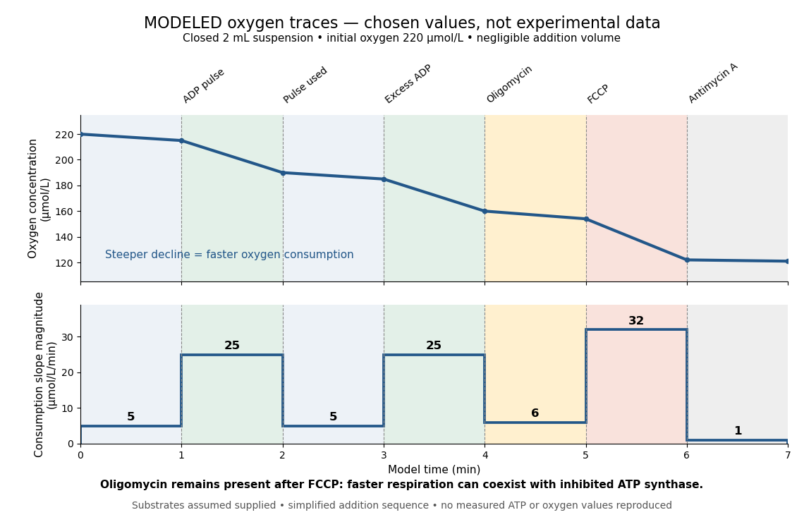
Start at $c(0)=220\mu \mathrm{mol}{\mathrm{L}}^{-1}$. On successive one-minute intervals, choose positive slope magnitudes $5,25,5,25,6,32,1\mu \mathrm{mol}{\mathrm{L}}^{-1}\mathrm{mi}{\mathrm{n}}^{-1}$. Integration gives the endpoint concentrations $220,215,190,185,160,154,122,121\mu \mathrm{mol}{\mathrm{L}}^{-1}$. This is just the recurrence $c_{i+1}=c_i-r_i\Delta t$, with $\Delta t=1\min$; the step plot shows $r_i=-dc/dt$. The trace remains above zero by construction.

During the second ADP interval, the total consumption rate isWith a stipulated mitochondrial protein mass of $0.20\mathrm{mg}$, that is $250\mathrm{nmol}\mathrm{mi}{\mathrm{n}}^{-1}\mathrm{m}{\mathrm{g}}^{-1}$. Using a denominator twice as large would halve this reported rate without changing the raw oxygen trace. Comparisons therefore need both loading and the chosen denominator.

For a second bookkeeping check, the modeled post-antimycin A slope of $1\mu \mathrm{mol}{\mathrm{L}}^{-1}\mathrm{mi}{\mathrm{n}}^{-1}$ corresponds to $2\mathrm{nmol}\mathrm{mi}{\mathrm{n}}^{-1}$ background. If that background is additive and unchanged in earlier windows, subtraction gives $48$, $10$ and $62\mathrm{nmol}\mathrm{mi}{\mathrm{n}}^{-1}$ for excess ADP, oligomycin and FCCP, respectively. The oligomycin-sensitive difference is $48-10=38\mathrm{nmol}\mathrm{mi}{\mathrm{n}}^{-1}$. It is a difference in oxygen consumption under the chosen interventions, not an ATP production rate. Converting it into one requires additional coupling assumptions or an independent ATP measurement; the FCCP interval shows why slope alone cannot supply that conversion.

Across the whole seven-minute example, consumption is $V(c(0)-c(7))=198\mathrm{nmol}$, also the sum of the seven interval consumptions. This equality checks the rate-to-amount accounting independently of how the intervals are named. Actual records require attention to calibration, mixing transients, background stability and decreasing oxygen availability; a line that steepens or flattens alone does not identify the cause.

Evidence transfers at a stated level. Sequence alignment can suggest a candidate relationship between genes; functional complementation tests whether a candidate can supply a particular function in a chosen recipient. Neither alone establishes identical native gene expression, identical signal transduction, or identical consequences in every species. The yeast cross-species complementation experiment is especially useful because it tests a conserved function by intervention rather than assuming it from resemblance. ^[ref]

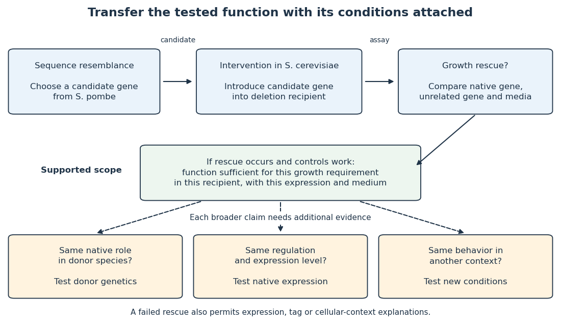
Even successful functional complementation occurs within a specific genetic background, nutrient supply and imposed gene expression. The enzyme may work with the recipient’s available substrates and partner proteins at an experimentally imposed abundance. Establishing the same role in the donor species calls for experiments there; establishing behavior under another condition calls for experiments under that condition. A conserved component can therefore coexist with context-dependent behavior of an entire pathway. This separation makes model organisms powerful: an accessible experiment supplies a precise mechanistic foothold and a better question for the next system.

A biologist who studies molecular mechanisms of living systems, especially how DNA, RNA and proteins store, express and regulate biological information. Reconstituting a process from selected components helps test which interactions are sufficient for an observed effect.

Molecular biology investigates biological processes through the structures, interactions and transformations of molecules. A central set of questions concerns how DNA and RNA participate in inheritance and gene expression, how biological translation produces proteins, and how those proteins influence cellular function. Molecular composition, sequence and physical interaction provide experimentally distinguishable kinds of evidence.

An important historical example is the1952 Hershey-Chase experiment. A. D. Hershey and Martha Chase compared the behavior of labeled DNA and labeled protein during infection by Bacteriophage T2. Phosphorus-32 and sulfur-35 supplied radioactive tracers associated with those different chemical components.^[ref]

The apparatus made physical location measurable. Agitation in a Waring blender detached externally attached phage material from infected bacteria; centrifugation separated cell-containing material from extracellular label. The investigators then compared label distributions and subsequent phage production. Differential transfer supported distinct roles for viral DNA and much of the sulfur-containing coat protein. It did not establish that every organism uses identical molecular machinery.^[ref]

An original fraction-accounting example makes the inference boundary explicit. If a corrected tracer assay gives120 units in one fraction and480 in another, the first contains $120/(120+480)=0.20$ of the recovered readout. That is a distribution of measured label under the assay assumptions. It is not automatically a20-percent contribution to heredity, cellular function or the number of molecules present. Label specificity, recovery and background determine what the measurement means.

The broader strategy is to connect a biological outcome with a manipulable molecular explanation. Sequence comparisons, structural observations and perturbations of gene expression answer complementary questions. A molecule can be present without being causally necessary for a tested outcome; changing it and measuring the consequence supplies a different kind of evidence. This combination links the study of biological cells with chemistry and quantitative experiments.

Molecular brightness is the detected fluorescence signal contributed by one labelled molecule or fluorescent particle under specified illumination and collection conditions. It is often expressed as detected photons per second per particle, or counts per particle per acquisition interval. It depends on the label, its environment and the apparatus, so it is not an intrinsic universal constant of the protein carrying the label.

For one uniformly observed species in a simple additive model, background-subtracted count rate $F$ and mean particle number $N$ satisfy $F=bN$, where $b$ is the molecular brightness. Ten particles with $b=1000$ counts per second and five particles with $b=2000$ counts per second both yield $F=10,000$ counts per second. Mean intensity alone cannot distinguish the two samples. A particle carrying two independent identical labels can approach twice the molecular brightness of one label, but quenching or incomplete labelling can invalidate that comparison.

Yan Chen and colleagues used the distribution of photon counts as particles diffuse through a tiny illuminated observation volume to estimate both molecular brightness and mean occupancy. This uses fluctuations beyond the average, with the illumination profile included in the measurement model.^[ref]

Investigation of disease using molecular features such as nucleic acid sequences or protein markers. Detecting a target and showing that it explains illness are distinct steps, especially when low-level or incidental material can be present.

Molecular evolution is inherited change in molecules such as DNA and proteins across generations. Mutations introduce new variants; natural selection and genetic drift influence which variants persist. Comparing a nucleotide sequence or protein sequence between lineages therefore supplies evidence about their history as well as their present chemistry.

An important early example was the comparison of cytochrome c from different organisms. Emanuel Margoliash's 1963 report connected differences in protein primary structure to evolutionary relationships. The experimental input was the ordered amino acid residues of the proteins, rather than only their bulk composition or their shared function. Placing corresponding positions side by side made molecular differences countable.^[ref]

For a deliberately simplified example, suppose two already aligned sequences have $k=8$ differing positions among $n=100$ compared positions. Their observed difference fraction is $k/n=0.08$. That statistic is not itself a divergence time. If both lineages split $t$ time units ago and each accumulates substitutions at the same constant rate $r$ per position per unit time, their expected accumulated pairwise molecular divergence isThe factor two counts the two descendant branches. At low divergence, the observed difference fraction can approximate $d$; repeated changes at one position can conceal earlier changes, and unequal branch rates invalidate the equal-rate simplification. A molecular clock additionally needs a rate or time calibration to turn molecular differences into dates.

Sequence identity is a measured agreement between aligned positions. homology is a historical relationship of common descent; it is not a percentage. Orthology and paralogy further distinguish relationships associated with lineage splitting and gene duplication. These distinctions matter when a phylogenetic tree is inferred from a chosen gene rather than directly observed.

The neutral theory of molecular evolution provides a complementary population-level explanation: molecular change need not always be an adaptive improvement. Motoo Kimura's 1968 argument emphasized the potential importance of neutral changes and genetic drift, while leaving room for natural selection.^[ref]

Molecular genetics studies the molecular basis of heredity, connecting DNA sequence, gene expression and phenotype. It asks how information is copied, expressed, regulated and altered. A change in a promoter can affect how much RNA is produced without changing the encoded protein sequence, whereas a coding mutation can change the product itself. Combining sequence analysis with controlled genetic perturbations helps distinguish correlation from a mechanism linking a genotype to an observed trait. ^[ref]

Molecular recognition is selective association between molecules through noncovalent interactions, often involving complementary shape and charge. A binding partner can distinguish chemically similar molecules without permanently joining them by a new covalent bond.^[ref]

A simple one-site chemical equilibrium model makes selectivity quantitative. Let a free ligand concentration be $L$, and let the dissociation constant of its complex with a binding partner be $K_d$. With independent sites and negligible depletion of free ligand, the bound fraction is $f=L/(K_d+L)$. For two partners with illustrative $K_d$ values of $1$ and $100\mu \mathrm{M}$, supplying $L=10\mu \mathrm{M}$ gives fractions $10/11\approx 0.91$ and $10/110\approx 0.091$.

Thus association can favor one partner strongly at a stated concentration. At very high ligand concentration, both fractions approach one, so selectivity in a practical measurement depends on conditions as well as binding constants. Affinity chromatography exploits this principle by attaching a ligand to a support and retaining selected proteins.^[ref] Recognition alone does not imply catalytic conversion or a downstream cellular response.

The molecular weight cut-off rates retention of reference molecules. One manufacturer's definition uses the mass at which approximately $90\%$ remains after seventeen-hour dialysis, tested with globular proteins. A $10\mathrm{kDa}$ rating uses dalton units: a mass, not a length or an absolute passage threshold.^[ref]

A semipermeable membrane has a distribution of passage sizes, and a molecule's shape affects passage as well as its mass. Near the nominal MWCO, slow passage can make substantial retention compatible with eventual leakage. The protein-retention experiment below makes retention an observable quantity rather than a universal yes-or-no property inferred from the label.

A morphogen is a signal whose spatial concentration helps specify different biological cell fates or behaviors during biological development. A morphogen gradient provides a positional cue: biological cells at different distances from a source experience different local concentrations and can follow different developmental pathways. A spatial concentration variation alone does not establish that a substance is a morphogen; its graded developmental effects matter. See Alberts et al., Molecular Biology of the Cell, 4th edition (2002): morphogens as graded developmental signals.

The beautiful idea is that one distributed signal can help organize several regions of a developing body. A continuous morphogen gradient can supply the input for distinct domains of gene expression, rather than requiring a separate signal for every position. A morphogen response threshold is a useful idealization of that interpretation: high, intermediate and low concentrations are assigned different outcomes. The morphogen reaction-diffusion equation describes one way to generate a morphogen gradient; the equation is a model of transport and reaction, while the morphogen is the signal being transported.

Detection and interpretation also depend on the receiving biological cell. For an extracellular morphogen, receptors and signal transduction connect the local concentration to a response; receptor binding occupancy is only one step in that connection. The same morphogen gradient can be interpreted differently in different tissues because their developmental context differs. Thus a morphogen response threshold summarizes a particular response in a particular context, rather than being a universal property of the signal. See Scott F. Gilbert, Developmental Biology, 6th edition (2000): positional information and context-dependent interpretation.

An important experimental example came in 1988. Wolfgang Driever and Christiane Nüsslein-Volhard used antibodies to examine the bicoid protein in early fruit-fly embryos. They reported a concentration profile approximately described by an exponential function, highest at the front, with the protein concentrated in cell nuclei. Their abstract proposed diffusion from localized messenger RNA and dispersed degradation as a likely origin of the morphogen gradient, rather than proving a unique transport mechanism. ^[ref]

In a companion study, Driever and Nüsslein-Volhard genetically changed the amount and distribution of bicoid messenger RNA, measured the resulting protein morphogen gradient, and compared developmental maps. Increased local bicoid protein levels shifted prospective anterior structures toward the rear; decreased levels shifted them toward the front. This linked a measured concentration profile to positional effects in biological development. The toy calculations below illustrate that logic with arbitrary numbers, not measured bicoid parameters. ^[ref]

A morphogen response threshold is a concentration level used to distinguish developmental responses to a morphogen. In an idealized threshold model, otherwise equivalent biological cells exposed to $c\ge \theta$ take one response and those exposed to $c<\theta$ take another. Two morphogen response thresholds can assign three bands: fate A for $c\ge 50$, fate B for $20\le c<50$, and fate C for $c<20$, all in the toy arbitrary concentration units. The A/B/C labels specify a response rule, not named cell types or a claim that every morphogen produces sharp boundaries. See the positional-information model in Gilbert's reference under morphogen.

For the decreasing morphogen gradient $c(x)=c_0{e}^{-x/\ell }$ and $0<\theta <c_0$, solve $c(x_{\theta })=\theta$ using the natural logarithm:With $c_0=100$ and diffusion length $\ell =100\mu \mathrm{m}$, the morphogen response thresholds $50$ and $20$ giveThus fate A occupies $0\le x\le x_{50}$, fate B occupies $x_{50}<x\le x_{20}$, and fate C occupies $x>x_{20}$ in this idealization. The equality convention belongs to the response rule. If $\theta =c_0$, the crossing is at the source; if $\theta >c_0$, that morphogen response threshold is never reached anywhere in the tissue.

Now double the prescribed source concentration from $c_0$ to $2c_0$, keeping $D$, $k$, diffusion length $\ell$ and a fixed morphogen response threshold $0<\theta <c_0$ unchanged. The whole morphogen gradient doubles, but the boundary moves by an additive distance:For $\theta =20$, the crossing moves from $160.9438\mu \mathrm{m}$ to $100\ln 10\mu \mathrm{m}\approx 230.2585\mu \mathrm{m}$, a shift of $69.3147\mu \mathrm{m}$. Every fixed morphogen response threshold below the original source concentration shifts by this same distance in the toy model. The example compares two Dirichlet boundary conditions, $c(0)=100$ and $c(0)=200$; doubling an experimentally supplied source flux is a different boundary specification.

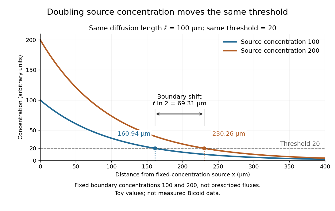
These calculations are useful because they separate changes in source concentration, diffusion length and response rule. Their limits are equally concrete: growing tissues change the geometry, a transient response can precede steady state, molecular fluctuations can blur a boundary, and signaling feedback or altered transport can change the morphogen gradient or its interpretation. A local instantaneous morphogen response threshold need not capture exposure duration, signaling adaptation or the receiving biological cell's state. Experiments on cultured human biological cells found different responses to the level and rate of change of developmental signals, illustrating why signal dynamics can matter. ^[ref] Quantitative measurements of bicoid protein and its downstream gene expression also make precision a question for experiment, rather than something guaranteed by drawing threshold lines. ^[ref] Morphogen gradients provide one mechanism for spatial patterning in biological development, alongside other signals and interactions.